Lagrange polynomials
I read a very nice article in the latest IEEE Signal Processing Magazine: Prandoni, P. and Vetterli, M., “From Lagrange to Shannon… and back: another look at sampling,” IEEE Signal Processing Magazine 26(5):138-144, September 2009. The authors make a case for teaching signal processing starting with discrete time, and then moving to continuous time. I don’t agree, but they expose their case very nicely. But I did learn something new from this paper, which is why I am writing this. It turns out that the Lagrange interpolation polynomials converge to the sinc function as the polynomial order goes to infinity.
Polynomial interpolation
Given a set of points , we want to find a continuous function such that . Creating such a function is called interpolation, and there are an infinite number of such functions. If we assume that the samples model some natural phenomenon, we can assume that the interpolating function we are looking for is smooth. Smooth means continuous and differentiable. This still leaves an infinite number of possibilities. To confine the options to just one function, we can require that the function be a polynomial of order , which has as many degrees of freedom as the number of samples in . A polynomial is infinitely differentiable, which means that not only is the function smooth, but its derivative is smooth, and the derivative’s derivative is smooth, and so forth. Constructing such a polynomial requires solving a set of equations, but can also be accomplished in a much simpler way: using the Lagrange basis polynomials of order :
where obtains each of the possible values of . These are the 5 Lagrange basis polynomials for :
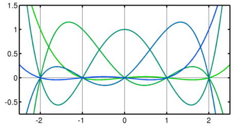
Note how each basis polynomial has a value of 1 for , and a value of 0 at all other sample locations. Simply multiplying each basis with the corresponding sample value, and adding them all up yields the interpolating polynomial:
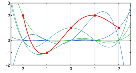
For example, these are the 5 weighted polynomials and their sum (red line) for a set of 5 random samples (red dots):
Interpolation through convolution
You can already see why we don’t use this when interpolating signals or images: you need to use all samples to interpolate, it is not a local operation. Plus, you get different interpolating basis functions depending on the number of samples in your image. More popular are the linear and cubic interpolators, which are short functions (zero for for linear, or for cubic), and you use a shifted version for each sample point. With these interpolating functions, the sum above becomes a convolution.
We’ve all learned that the sinc function is the ideal interpolator, and this is usually shown by its characteristics in the Fourier domain. Much like the linear and cubic interpolators, shifted versions of the sinc function form the basis functions that, weighted and summed, form the interpolating function. But unlike these, it is infinitely differentiable and has an infinite extent. These are some of the same characteristics that the Lagrange basis polynomials have. And, as it turns out, when the Lagrange basis polynomials are shifted versions of the sinc function! There is a rigorous proof in the paper I reference above, involving Fourier series and awkward trigonometry. But you can see that this might be true just looking at one Lagrange basis polynomial with a high order, (the green line is the sinc function):
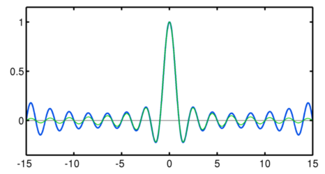
The polynomial actually becomes increasingly larger for larger , which is weird, but remember that 100 is very far away from infinity. The higher the order, the larger the area over which this is a good match.
The need for smoothness
So this paper uses this equivalence to argue that we should teach signal processing starting in the discreet domain. To interpolate, an infinitely differentiable function is required because
Nature […] abhors abrupt jumps, either in magnitude or slope.
Thus, the sinc is the only function that makes sense to interpolate with. Using this interpolator we obtain a band-limited, continuous-domain signal. This argument turns the sampling theorem upside-down. It is a nice idea, but there is one problem: the argument as to why we need an infinitely differentiable interpolator is very weak. Nature might abhor abrupt jumps, but they certainly happen. There exists such a thing as an interface in physics (which, by the way, is difficult to model because it can’t be sampled!). Many properties are either discontinuous at an interface, or their first or second derivative is. Unless you impose the requirement of bandlimitness to a function before you sample it, there is no reason to assume that a set of samples needs to be interpolated using an infinitely differentiable function. This is why I’m still teaching the sampling theorem starting in the continuous domain.