Cris’ Image Analysis Blog

We recently organized the 11^th International Symposium on Mathematical Morphology here in Uppsala. I’m very happy with how the event turned out, and we got lots of positive comments from participants, so all our hard work paid off. We had a nice turnout, very interesting presentations, and lots of discussions. And I’m now the editor of a book containing all the papers presented.

There seem to be several trending topics in the ISMM community at the moment. One of those is the application of Mathematical Morphology to colour images. People have been working on this topic for a while now, and still there is no optimal solution. This year, three very different methods were presented to try and solve this problem. But what is this problem about?

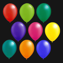
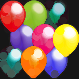
When applying linear filters to an image, for example a Gaussian smoothing, one computes the weighted average of a set of pixels. Averaging colours works fine, and is trivial in the sense that it is computed by averaging each of the colour components separately. For example, in the RGB colour representation, the value of each pixel is given by a three-dimensional vector, [r, g, b], where the r value gives the amount of red, g the amount of green, and b the amount of blue. Thus, the colour value is a point in the three-dimensional RGB space. Averaging two of these values is the same as averaging each of their components. The average of a yellow pixel and a red pixel is an orange pixel. This produces results that we expect and look natural:

a = readim('baloons.png')
s = 25;
b = gaussf(a,s/2)

However, Mathematical Morphology is based around partial ordering of pixel values. What this means is that, for any set of pixels, we need to be able to find the lowest-valued one and the highest-valued one. And here is the problem: what is larger, red or yellow? There is no natural ordering of colours, as hue is a circular property: we can link the top and the bottom of the rainbow by adding purple. That is, one can order the colours in a circle like so: red, yellow, green, blue, purple, red, … Both saturation and intensity (brightness) have a clear ordering, but hue does not. And this is a property of the colours themselves, independent of the numerical representation (colour space) we use.

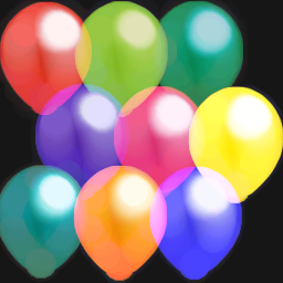
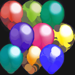
Computing a Mathematical Morphology operation component by component (referred to as marginal ordering) produces unexpected results: new colours are created, which gives all sorts of problems in Mathematical Morphology. New colours are also not always expected: the maximum of red and green is yellow, the maximum of yellow and blue is white, and the maximum of green and yellow is yellow:

c = iterate('dilation',a,s)

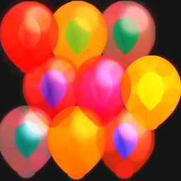
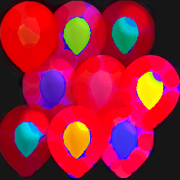
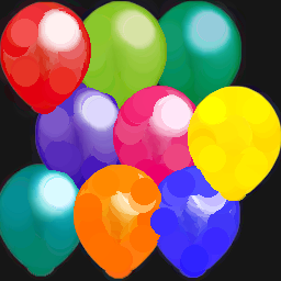
Using a different colour space does not solve this issue, though the result is different for each colour space. For example in CIE-Lab and HSV colour spaces the same operation produces these results:

c2 = iterate('dilation',colorspace(a,'lab'),s)

c3 = iterate('dilation',colorspace(a,'hsv'),s)

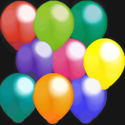
Thus, clearly, we need to treat the pixel values as a vector, not three independent values. Classical solutions are many. The simplest one is to sort the vectors according to the first component, for vectors with identical first component, sort according to the second, etc. This is called lexicographical ordering, as it is the same process that is used to sort words in a dictionary (also often referred to as conditional ordering). This means that a pixel with a medium red intensity is larger than one with a low red intensity, even if that second pixel has a very high green intensity. This yields a strong bias towards the red:

mergechannels = @(in)(round(in{1})*(256*256)+...
                      round(in{2})*256+round(in{3}));
d = mergechannels(a);
d = iterate('selectionf',a,-d,s)

We can do the same thing but sorting according to the blue intensity first:

d2 = mergechannels(a{[3,1,2]});
d2 = iterate('selectionf',a,-d2,s)

Lexicographical ordering works better in a different colour space. Sorting on intensity first, then saturation, and finally hue, one obtains this result:

d3 = colorspace(a,'hsv').*[255/6,255,1];
d3 = mergechannels(d3{[3,2,1]});
d3 = iterate('selectionf',a,-d3,s)

You’ll agree with me that lexicographical ordering does not produce nice results in these cases. This is true in general. Another simple solution to the ordering of colours is not to try to always order them all. One can pick one property, usually intensity, and sort on that, ignoring the actual colours. If two pixels with different colour values but same intensity are found, the dilation can pick the colour closest to the origin of the structuring element (centre of the filter window). The result would look like this:

e = iterate('selectionf',a,-colorspace(a,'grey'),s)

Still not a perfect result, but much better than using lexicographical ordering. Most of the more complex approaches are based on this principle, called reduced ordering. The trick is to find an axis in the colour space, other than the intensity, that is relevant for the image being processed. For example, if the blue sky is being considered the background, and the foreground is a red balloon, then an appropriate axis would go from blue to red. The distance to a chosen colour can also be used for reduced ordering. A still up-to-date overview by Aptoula and Lefèvre from 2007 will give a broader overview (PDF).

One of the approaches presented this year at ISMM was based on this principle, the authors used Principal Component Analysis (PCA) to find a relevant axis. The novel aspect of their paper was that they then used the distance to the extrema estimated by PCA to impose an ordering. The two other approaches presented were more complex. One involved frames and the other involved matrices, cones and mathematics used by Einstein when he worked with relativity theory.

The approach using frames requires transforming the colours in all ways that you want the operator to be independent of, compute the operation on all these transformed images (using marginal ordering), and then compose all the results into a single image. By computing the operation on all these transformations, you make sure that the result is identical if the input image is transformed in a similar way. For example, if you include all possible rotations of the hue channel in the operation, the result of the operation will not prioritize any hue over any other hue, and the result will be identical if objects change colour.

The third approach does not try to impose an ordering on colours, recognizing that it is not possible, and instead tries to find a colour that is considered larger than all colours under the mask. It does this by embedding the colour information (a vector) into a symmetric, positive definite matrix, and applying the Loewner order. This ordering allows determining a matrix that is larger than all the matrices in a set by finding the smallest cone of positive semidefinite matrices that contains the set; the tip of the cone represents the matrix that is larger than all the matrices in the set. The problem here is that, given two colours, the resulting maximum can be outside the cone generated by those two colours and a third one. That is, if d = max(a,b), then max(a,b,c) ~= max(d,c). To solve this problem, the space in which the cones are defined is warped so that the cones become half-spheres. When using the same mathematics as used in Einstein’s Relativity Theory, the addition in this space never results in values outside the unit circle, and thus never produce non-existent colours. I was quite impressed with the large collection of diverse mathematical concepts this paper collects to solve the problem, but am presuming that the operations proposed are too complex for efficient implementations. However, do note that these operations will also be useful on complex data such as diffusion tensor MRI, which produces positive definite matrices as pixel values.

I am not showing results for these three methods, I wish I had time to implement these ideas!