DIPimage 2.5.1 released
We recently released a bugfix for DIPimage release 2.5. Since I didn’t announce the release of 2.5 here, this might be a good opportunity to review some of the improvements in 2.5.
The Fourier transform
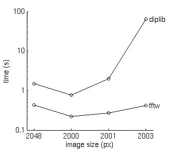
One of the most important changes, in my mind, was also quite simple to implement: we added an option to use MATLAB’s built-in FFT functions instead of the one in DIPlib. MATLAB’s built-in functions use the FFTW library (“Fastest Fourier Transform in the West”). Here I compare the execution time on a reasonably large image (20482 pixels) and three cropped versions of it: 20002, 20012 and 20032 pixels. This last image size is a prime number. If you know about the Fast Fourier Transform algorithm, you know that sizes that are a power of two are the fastest to compute because you can halve the size until you have a single pixel left. A round number like 2000 is easily decomposed into favourable sections, and a prime number requires the most complex code to efficiently compute the FT. Not surprisingly, it is for the prime image size that the DIPlib code is the least efficient (FFTW is two orders of magnitude faster!); but also for the nice image sizes, DIPlib needs about three times as much time as FFTW to do the computations. Here is the code and a little graph comparing the results:
clear all
a = repmat(readim,[8,8]); % a power of two number of pixels
b = a(0:1999,0:1999); % a round number of pixels
c = a(0:2000,0:2000); % an odd number of pixels
d = a(0:2002,0:2002); % a prime number of pixels
t = zeros(4,2);

dipsetpref('FFTtype','diplib')
t(1,1) = timeit(@() ft(a));
t(2,1) = timeit(@() ft(b));
t(3,1) = timeit(@() ft(c));
t(4,1) = timeit(@() ft(d));

dipsetpref('FFTtype','fftw')
t(1,2) = timeit(@() ft(a));
t(2,2) = timeit(@() ft(b));
t(3,2) = timeit(@() ft(c));
t(4,2) = timeit(@() ft(d));

clf
set(gcf,'position',[300,300,340,300])
set(gca,'fontsize',12,'linewidth',1)
plot(t,'ko-','linewidth',1)
set(gca,'xtick',1:4,'xticklabel',{size(a,1),size(b,1),size(c,1),size(d,1)},'xlim',[0.8,4.2])
xlabel('image size (px)')
ylabel('time (s)')
set(gca,'yscale','log','ylim',[0.1,100],'yticklabel',[0.1,1,10,100]);
box off
text(4.1,t(4,1),'diplib','fontsize',12)
text(4.1,t(4,2),'fftw','fontsize',12)
print -r0 -dpng fft_test.png
Note that I’ve used the function timeit, which is included with MATLAB since version 2013b (just released).
If you have an older version of MATLAB (like I do), get this function from the MATLAB File Exchange.
Arithmetic
Several internal changes to how arithmetic operations are resolved (not the actual code that does the computations) were
introduced in release 2.5. These changes also introduced some unintended changes in behaviour (i.e. bugs), which
were fixed in release 2.5.1. One of the problems that prompted
us to make these changes was that it was impossible to make a scalar image of type other than 'sfloat' (even
when 'dfloat' was explicitly requested, the number was converted to single precision first, then converted back to
double precision, meaning that precision was lost). A consequence of the changes is that the function dip_arith, which
is called to compute the output of arithmetic operations, now has an additional input parameter to select the data type
of the output. You can exploit this new parameter to avoid the default behaviour where the output of an arithmetic
operation is always a floating point type. For example, consider a and b two images of type 'uint8' (8-bit
unsigned integers). The code
c = a+b;
produces an image c that is of type 'sfloat'. This is an easy way of avoiding overflow errors, as well as rounding
errors in the multiplication and division. Now you can instead type
c = dip_arith(a,b,'add','uint8');
and obtain an image c that is of type 'uint8'. The main advantage here, of course, is the memory saved (1 byte per
pixel instead of 4 bytes per pixel).
(PS: Actually, dip_arith is a new function. Previously we had dip_add, dip_mul, etc., but the underlying DIPlib
code called is the same.)
Other improvements
We have a few more improvements, see the full changelists for release 2.5
and release 2.5.1. For example, reading TIFF stacks as a
single 3D image is much faster now, and we added Lanczos interpolation to the options in resample and rotation (the
options are called 'lanczos2', 'lanczos3', 'lanczos4', etc. for the various useful values of parameter a in the
method).