Gaussian filtering
In my recent lectures on filtering I was trying to convey only one thing to my students: do not use the uniform filter, use the Gaussian! The uniform (or “box”) filter is very easy to implement, and hence used often as a smoothing filter. But the uniform filter is a very poor choice for a smoothing filter, it simply does not suppress high frequencies strongly enough. And on top of that, it inverts some of the frequency bands that it is supposed to be suppressing (its Fourier transform has negative values). There really is no excuse ever to use a uniform filter, considering there is a very fine alternative that is very well behaved, perfectly isotropic, and separable: the Gaussian. Sure, it’s not a perfect low-pass filter either, but it is as close as a spatial filter can get.
Because recently I found some (professionally written) code using Gaussian filtering in a rather awkward way, I realized even some seasoned image analysis professionals are not familiar and comfortable with Gaussian filtering. Hence this short tutorial.
First of all, for reference, this is the equation for a Gaussian:
An isotropic multi-variate Gaussian is defined as (with an -dimensional vector):
Scaling the various axes can be accomplished giving a different for each dimension. For example, in two dimensions this gives:
The Gaussian as a Smoothing Filter
The Gaussian can be used as a smoothing filter. Its Fourier transform is a Gaussian as well, with a sigma of , meaning it strongly suppresses frequencies above . What is more, it is monotonically decreasing for increasing , like a good smoothing filter should be, and real and positive everywhere, meaning the filter does not change the phase of any frequency components. Even thought the Gaussian does not have a cutoff frequency, its Fourier transform is very close to zero after certain value of , meaning it can be sampled with only a very small error if is larger than 0.9 or so.
This demo gives a good indication of what is wrong with the uniform filter:
a = cos(phiphi*100) * erfclip((rr-40)/2,0.5,1);
b = unif(a,9,'rectangular');
c = unif(a,9);
d = gaussf(a,3);
a =   a(  0:127,  0:127);
b = 4*b(128:255,  0:127);
c = 4*c(128:255,128:255);
d = 4*d(  0:127,128:255);
dipshow(clip((1+[a,b;d,c])*(255/2)))
hold on
plot([0,255],[128,128],'k')
plot([128,128],[0,255],'k')
text(120,120,'a')
text(136,120,'b')
text(136,140,'c')
text(120,140,'d')
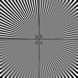
a is a test image with a line pattern that decreases in frequency as one moves from the center to the edge. b is
filtered with a uniform filter with a 9x9 rectangular support. c is a uniform filter with a circular support. It shows
the same characteristics, but is much more isotropic. d is filtered with a Gaussian. Note how the uniform filter
inverts the line pattern at various points in the image.
Computing Derivatives
The derivative of a function is defined as its slope, which is equivalent to the difference between function values at
two points an infinitesimal distance apart, divided by that distance. On a discrete grid, the smallest distance
obtainable without interpolation is 1. This yields the finite difference approximation of the derivative: a linear
filter with values [1,-1]. This approximation actually computes the derivative in between the two grid points, meaning
that the output of the filter is shifted by half a pixel. This is often solved by using a distance of 2 instead of 1. We
now have a filter [1,0,-1]/2, which is odd in size.
The problem with these filters is that they respond very strongly to noise. Hence the introduction of filters like
Prewitt and Sobel, that add some smoothing in the direction orthogonal to the derivative direction. Of course, these
filters had to use a uniform or a triangular filter, instead of a good smoothing filter. (The triangular filter has
better properties than the uniform filter, but does not suppress high frequencies as well as the Gaussian.) But even if
we ignore the poor choice of smoothing filter, this type of derivative operator is in general a bad idea. Why? Because
each of the components of a gradient vector computed with these filters has a different smoothing. Let me explain this.
A filter like Prewitt is separable, equivalent of applying the [1,0,-1]/2 along one axis, and the [1,1,1]/3 filter
along the other axis. So basically we are computing the partial derivative along the x-axis of an image that was
smoothed with a 1x3 uniform filter, and then computing the partial derivative along the y-axis of an image that was
smoothed with a 3x1 uniform filter. The two partial derivatives are derivatives of different images! Needless to say, if
we combine these into one gradient vector we obtain a nonsensical result (or a poor approximation at best). This means
that these filters are not rotation invariant.
So what is so great about those “Gaussian derivatives” I keep hearing about? Don’t they do the same basic thing as Prewitt and Sobel, but with a proper smoothing? Well, yes, but there is more. We learned above that the derivative is a convolution. We also know that the convolution is associative and commutative. These properties show us that computing the gradient of an image blurred with a Gaussian is the same thing as convolving the image with the gradient of a Gaussian:
And because we can compute the derivative of the Gaussian analytically, and because it has a bandlimit similar to that of the Gaussian itself, we can sample it and make a filter out of it. What is so exciting? We are now computing the exact gradient of a blurred version of our image. This is no longer a discrete approximation to the gradient, but an exact analytical gradient. Of course, we cannot compute the gradient of the image itself, only of its blurred version, which means we are still approximating the gradient. But in any application that requires accurate gradients, we needed to blur the image anyway because the gradient is so noise sensitive.
Convolutions with a Gaussian
One very important theorem in all the sciences is the central limit theorem. OK, officially it belongs to statistics, but this theorem is the reason we all have to deal with Normally distributed noise. It states that, if we add together a large enough set of random variables with whatever distribution, the resulting random variable is normally distributed. The Gaussian emerges again and again as a probability distribution in nature, Brownian motion is a classic example. The central limit theorem also tells us that, if we convolve any compact filtering kernel with itself often enough, we obtain a Gaussian kernel. Meaning that by convolving an image repeatedly with a uniform filter we can approximate a Gaussian filter. It also means that convolving an image twice with a Gaussian filter yields an image filtered with a larger Gaussian filter. The size parameter of this resulting larger Gaussian filter can be computed by quadratically adding the s of the applied filters: . So when repeatedly convolving an image with the same Gaussian, we effectively increase the with a factor √2 with every convolution. Note that this is independent of the order in which the gradient convolution is applied: the convolution is commutative. This means that if we smooth the image with a Gaussian of , then compute a gradient with a Gaussian derivative of , we could just as well have computed the gradient straight away, using a Gaussian derivative of .
Furthermore, because the Gaussian is separable, you can compute the convolution with a 2D Gaussian by applying 1D convolutions, first along each of the rows of the image, then along each of the columns of the result:
Or first along the columns and then along the rows, whatever floats your boat. And of course you can do this in your 5D image just as nicely as in a 2D image. But more importantly: this is also true for the gradient!
What I’m saying here is that you, yes, you who wrote that code that nicely smoothed the image with a 1D Gaussian first along rows and then along columns, and then computed the x and y derivatives by applying full 2D convolutions with 2D Gaussian derivatives, you were wasting a lot of computer clock cycles. Skip the first blurring, you don’t need it, and compute the gradient as the separable convolution that it is. Please.