Panoramic photograph stitching
I found the article “Fast image blending using watersheds and graph cuts,” by N. Gracias, M. Mahoor, S. Negahdaripour and A. Gleason (Image and Vision Computing 27(5):597-607, 2009) quite clever, and decided to try it out myself. Here’s a little demo and the code I wrote.
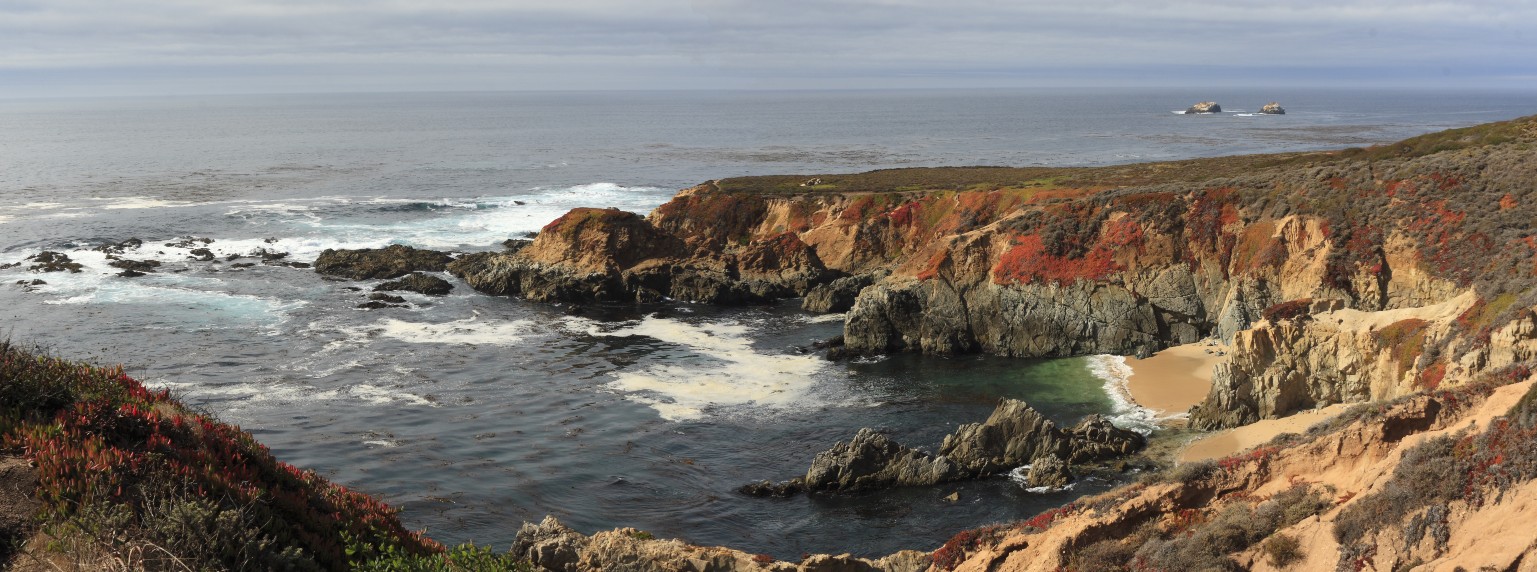
I had these two images lying around, that I took some years ago at Big Sur:
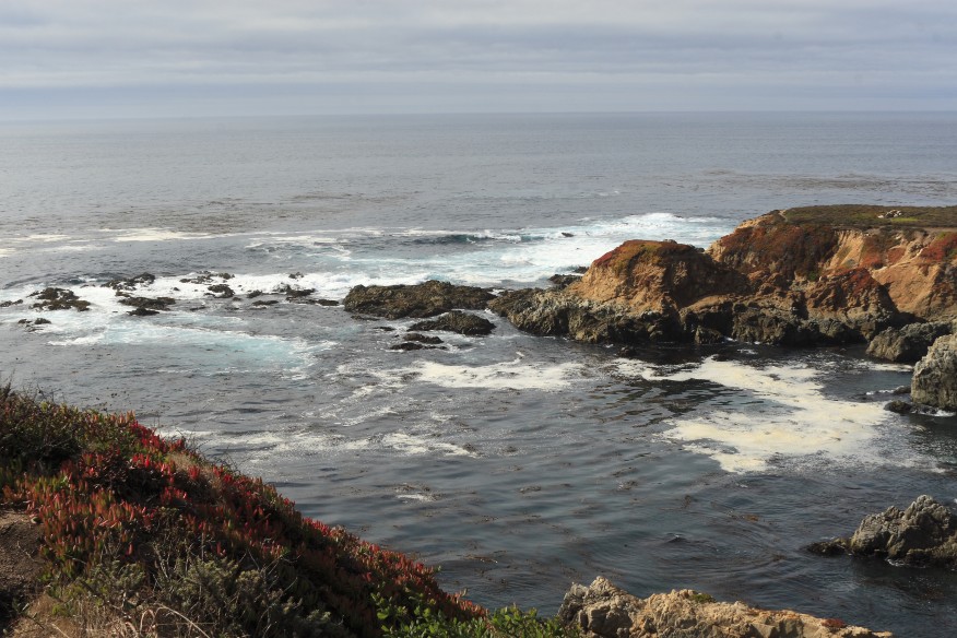
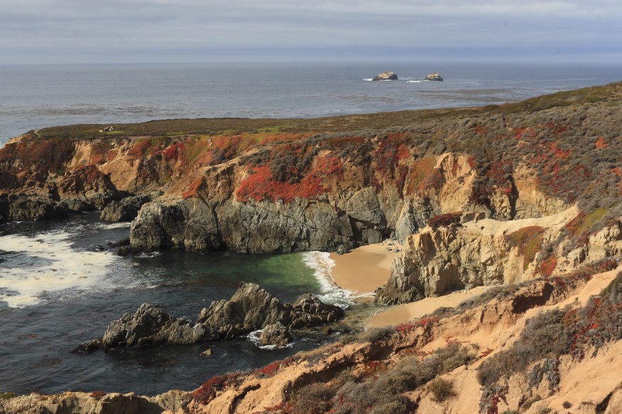
I’m not bothering with warping the images to undo the projection, so only one point in the two images can be correctly
aligned. This actually makes it easier to see the effect of this method. I read them into the variables a and b.
The first job is to find that common point. I used the DIPimage command dipgetcoords to get
the coordinates of a mouse click in each image. I clicked on one small rock towards the middle of the area of overlap of
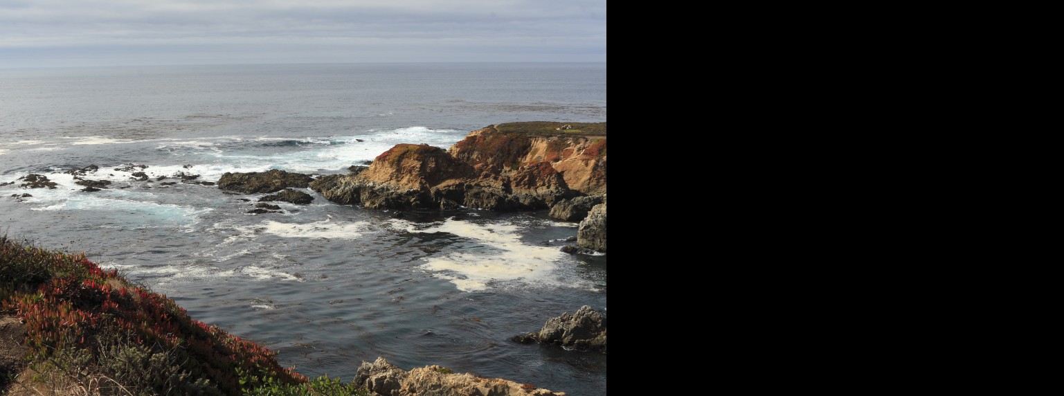
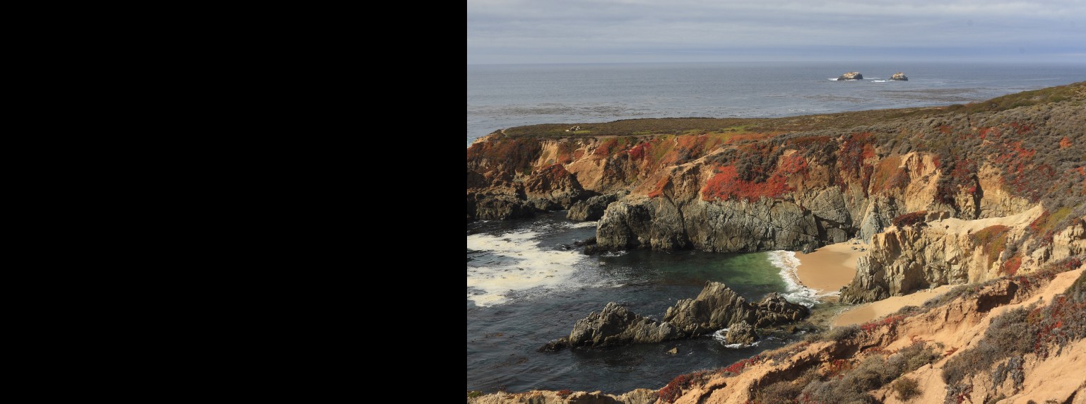
the two images. Next I expanded and shifted the two images:
sz = imsize(a);
dipshow(1,a);   ca = dipgetcoords(1,1);
dipshow(1,b);   cb = dipgetcoords(1,1);
s = ca - cb - [sz(1),0];
z = newim(sz);
a = iterate('cat',1,a,z);
b = iterate('cat',1,z,b);
b = iterate('dip_wrap',b,s);  % For DIPimage 2, in DIPimage 3 use `wrap` rather than `dip_wrap`
Note how in DIPimage you sometimes need to use iterate to work with color images. [Note: In DIPimage 3 this is
less often the case, and both cat and wrap work on color images.]
The next step is to look at the inverse of the absolute difference between the two images. I set the inverse difference to 0 in the areas where only one image is available.
d = 255 - max(abs(a-b));
d(0:sz(1)-1+s(1),:) = 0;
d(sz(1):imsize(d,1)-1,:) = 0;

In the paper they apply a watershed to the blurred difference image. They use the blur to avoid getting too many regions: every single local minimum produces a region, and even small amounts of noise create an inordinate amount of local minima. The watershed function in DIPimage has built-in region merging, so this blur is not necessary. I’m using the low-level interface to the watershed algorithm because it has the option of returning a labeled image of the watershed regions instead of a binary image of the watershed lines:
w = dip_watershed(d,[],1,50,1e9,0);      % For DIPimage 2
% w = watershed(d,1,50,1e9,{'labels'});  % For DIPimage 3

The image above shows the watershed lines (right-click the image and select “view image” to get a closer look), but the
image w computed above is a labeled image.
The next step is to generate a graph in which each node represents one of the watershed regions, and the edges are the
gray-value of the image d in between the regions. The paper uses the maximum difference between the two regions
(lowest grey-value). However, I got better results using the integrated grey-value over the boundary between the two
regions. This way it takes the difference in boundary lengths into account. The code to compute this is rather slow and
inelegant, but it does the job:
labs = unique(double(w));
labs(1) = [];     % labs == 0 doesn't count
N = length(labs);
V = zeros(N,N);   % vertices
for ii=1:length(labs)
   m = w==labs(ii);
   l = unique(double(w(bdilation(m,2,1,0))));
   l(1) = [];     % l == 0 doesn't count
   l(l==labs(ii)) = [];
   for jj=1:length(l)
      kk = find(l(jj)==labs);
      if V(ii,kk) == 0
         n = w==l(jj);
         n = closing(m|n,2,'rectangular') - m - n;
         if ~any(n)
            V(ii,kk) = 0.01;
         else
            V(ii,kk) = sum(d(n));
         end
         V(kk,ii) = V(ii,kk);
      end
   end
end
The code above generates a matrix V, in which V(i,j) is the weight of the edge between vertices i and j. labs
is the list of labels used in the image w, such that vertex i has label ID labs(i). The code loops over all
labels, extracts the area corresponding to one label, and applies a small dilation to find label IDs of the neighboring
regions. Then, looping over each neighbor, it finds the area in between the two regions and integrates the gray-values
of d.
According to the paper, the max-flow/min-cut of this graph is the ideal line over which to stitch the two images
together. To compute the max-flow/min-cut line I downloaded the
package maxflow by Miki Rubinstein from the MATLAB File
Exchange. The big regions on the left and right side of the image will be the source and sink for computing the flow.
The following bit of code finds the label IDs for these two regions and removes them from the matrix V. An array T
is created with the two deleted columns, it shows which vertices are connected to the source and sink:
N1 = double(w(1,1));
N2 = double(w(end-1,1));
kk1 = find(labs==N1);
kk2 = find(labs==N2);
T = [V(:,kk1),V(:,kk2)];
V([kk1,kk2],:) = [];
V(:,[kk1,kk2]) = [];
T([kk1,kk2],:) = [];
labs([kk1,kk2]) = [];
[flow,L] = maxflow(sparse(V),sparse(T));
The matrix L contains 0 or 1 for each vertex, indicating whether it is connected to the source or the sink. I now
color each region in the image w with the correct label ID, then propagate labels to remove all the unassigned
pixels (the watershed lines):
w = setlabels(w,labs(L==0),N1);
w = setlabels(w,labs(L==1),N2);
w = dip_growregions(w,[],[],1,0,'low_first');  % For DIPimage 2
% w = growregions(w,[],1,0);                   % For DIPimage 3
w = w==N2;

The final composition is trivial using this mask:
out = a;
out(w) = b(w);
For comparison, I’ve stitched the image in two other ways: One is a dumb method, pasting the two images together with a straight line. Another is the method you see everywhere, also using a straight line, but blending the two images together using a little bit of blurring:
m = newim(w,'bin');
m(round(imsize(m,1)/2):end,:) = 1;
out_dumb = a;
out_dumb(m) = b(m);
m = gaussf(m,3);
out_common = a*(1-m) + b*m;
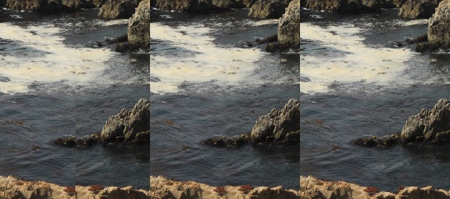
As you can see, the blurring (middle) hides the joint quite well, but it can be really obvious if there’s larger differences between the two images across the joint. The new method (right) makes it really difficult to see where the images were stitched. Because of the lack of alignment of the two images, some rocks can be seen twice in the stitched image. Oh well.
Feel free to download the script I used to generate the images on this page. [Note: This script was written for DIPimage 2, and will not work unmodified with DIPimage 3. See the comments in the code in this post for how to change the script.]
Edit April, 2011
For a simpler, faster method to accomplish more or less the same thing, see this new post.