The Laplacian of Gaussian filter
The Laplacian of Gaussian filter (LoG) is quite well known, but there still exist many misunderstandings about it. In this post I will collect some of the stuff I wrote about it answering questions on Stack Overflow and Signal Processing Stack Exchange.
What does it do?
From my answer to the question “Is Laplacian of Gaussian for blob detection or for edge detection?”
Very often I see the LoG described or referred to as an edge detector. It is not. A detector is a filter that yields a strong response at the location of the thing to be detected. The LoG has zero crossings at (or rather near) edges. However, it can be used to construct an edge detector. The edge detector so constructed is the Marr-Hildreth edge detector. This is likely what causes confusion. The LoG is a line detector.
Because (as we’ll see in detail later) the LoG is the sum of second derivatives, and the second derivative is large at extrema, the LoG will have large values at extrema (maxima or minima) along at least one dimension. This happens at the peak of a “blob” and along the ridge of a line.
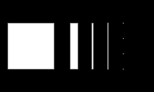
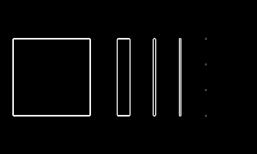
Let’s take this simple test image:
and apply the LoG to it:
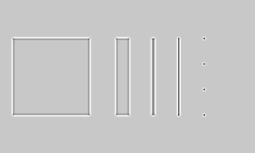
Here, mid-gray are pixels with a value of 0. As can be seen, it has strong (negative) response along the thin line and on the small dots. It also has medium responses around the edges of the wider objects (negative inside the edge, positive outside); the zero crossings are close to where the edges are.
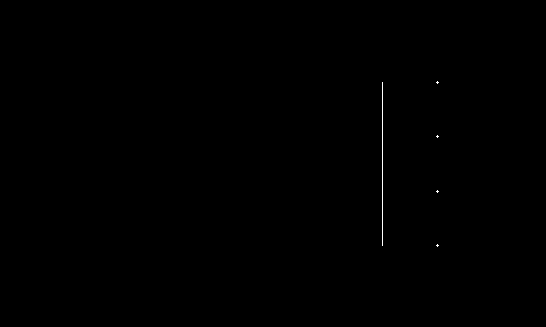
We can threshold this image to detect the thin line and the dots:
(thresholding the magnitude yields the same result). We can lower the threshold to see that medium responses happen around edges of interest:
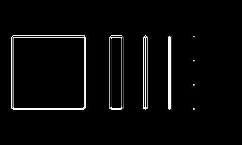
It takes more than a simple threshold to obtain edges. In contrast, the gradient magnitude can be thresholded to obtain edges (first derivatives are strong at the location of edges):
The gradient magnitude is not useful to detect lines, as it detects the two edges along the lines, rather than the line itself. Note that the Canny edge detector is based on the gradient magnitude, it adds non-maximum suppression and hysteresis thresholding to make the detections thin and meaningful.
How is it defined?
From my answer to the questions “How is Laplacian filter calculated?”, “Laplacian kernels of higher order in image processing”, and “What is the difference between Difference of Gaussian, Laplace of Gaussian, and Mexican Hat wavelet?”
The LoG filter is defined as the Laplace operator applied to a Gaussian kernel. The Laplace operator is the sum of second order derivatives (i.e. the trace of the Hessian matrix),
Derivatives of an image are hard to compute (the finite difference approximation is too sensitive to noise), so often we use Gaussian regularization when computing these derivatives. When applied to the Laplace operator, Gaussian regularization leads to the LoG:
(with the image and the Gaussian kernel, and the convolution operator). What this equation says is that the Laplacian of the image smoothed by a Gaussian kernel is identical to the image convolved with the Laplacian of the Gaussian kernel.
How is it computed?
From my answer to the questions “How Is Laplacian of Gaussian (LoG) Implemented as Four 1D Convolutions?”, and “A faster approach to Laplacian of Gaussian”
The Laplace of Gaussian is not directly separable into 1D kernels. Therefore, determining its full kernel and applying
it as a single convolution (e.g. in MATLAB using the imfilter function) will be quite expensive. But we can manually
separate it out into simpler filters.
From the equations above we can derive
The Gaussian itself, and its derivatives, are separable. Therefore, the above can be computed using four 1D convolutions, which is much cheaper than a single 2D convolution unless the kernel is very small (e.g. if the kernel is 7×7, we need 49 multiplications and additions per pixel for the 2D kernel, or 4·7=28 multiplications and additions per pixel for the four 1D kernels; this difference grows as the kernel gets larger). The computations would be:
sigma = 3;
cutoff = ceil(4*sigma);
G = fspecial('gaussian', [1,2*cutoff+1], sigma);
d2G = G .* ((-cutoff:cutoff).^2 - sigma^2) / (sigma^4);
dxx = conv2(d2G, G, img, 'same');
dyy = conv2(G, d2G, img, 'same');
LoG = dxx + dyy;
If you are really strapped for time, and don’t care about precision, you could set cutoff to a smaller multiple
of sigma (for a smaller kernel), but this is not ideal.
There is an alternative, less precise, way to separate the operation:
(with the Dirac delta, convolution’s equivalent to multiplying by 1). That is, we first apply the Gaussian regularization to the image, then compute the Laplacian of the result. The operator doesn’t really exist in the discrete world, but you can take the finite difference approximation, which leads to the famous 3×3 Laplace kernel (see my answer to the question How is Laplacian filter calculated?):
    [ 1  1  1             [ 0  1  0
      1 -8  1       or:     1 -4  1
      1  1  1 ]             0  1  0 ]
Now we get a rougher approximation, but it’s faster to compute (two 1D convolutions, and a convolution with a trivial 3×3 kernel):
sigma = 3;
cutoff = ceil(3*sigma);
G = fspecial('gaussian', [1,2*cutoff+1], sigma);
tmp = conv2(G, G, img, 'same');
h = fspecial('laplacian', 0);
LoG = conv2(tmp, h, 'same'); % or use imfilter
What is its relationship to the Ricker wavelet, the Mexican hat operator?
From my answer to the question “What is the difference between Difference of Gaussian, Laplace of Gaussian, and Mexican Hat wavelet?”
The Ricker wavelet or Mexican hat operator are identical to the Laplacian of Gaussian, up to scaling and normalization, though they are typically defined in 1D.
What is its relationship to the Difference of Gaussian?
From my answer to the question “What is the difference between Difference of Gaussian, Laplace of Gaussian, and Mexican Hat wavelet?”
The Difference of Gaussians (DoG) is similar to the LoG in its uses. In fact, the DoG can be considered an approximation to the LoG. However, these two filters are not identical in general, as the DoG is a tunable band-pass filter where both the center frequency and the bandwidth can be tuned separately, whereas the LoG has a single parameter that affects both the center frequency and the bandwidth simultaneously. It is possible to demonstrate the equivalence (up to scaling) of the LoG and DoG, if taking the difference in sigma between the two Gaussian kernels to be infinitesimally small.
The DoG of image can be written as
So, just as with the LoG, the DoG can be seen as a single non-separable 2D convolution or the sum (difference in this case) of two separable convolutions. Seeing it this way, it looks like there is no computational advantage to using the DoG over the LoG.
I once read a paper where the authors derived a separable approximation to the DoG kernel, reducing computational cost by half. Though that approximation was not isotropic, leading to rotational dependence of the filter. (I can’t seem to find this paper now.)