Cris’ Image Analysis Blog

DIPlib 3.1.0 was released last week (see the change log). One of the changes in this release is a very significant speed improvement in the morphological reconstruction (dip::MorphologicalReconstruction). This is quite an interesting story, so I decided to write it down.

The morphological reconstruction algorithm can be described as an iterative dilation or erosion of an image f conditioned by an image g. That is, we iterate the following statement until the image f doesn’t change any more:

f = min(dilation(f, 3), g);

Of course this can be implemented much more efficiently. In 1993, Luc Vincent (on a roll publishing efficient algorithms for quite a few morphological operators, including the watershed) published a paper describing four possible implementations of the reconstruction operator [1]. The fourth method, the most efficient one, is a combination of two other methods: first it does a raster and an anti-raster scan (see box below for an explanation), then it uses a FIFO queue to complete the propagation. In 2004, Robinson and Whelan published a paper describing a much more efficient algorithm, based on a priority queue [2]. This table from the paper shows the results of experiments on 2D images (there’s a similar one for 3D):

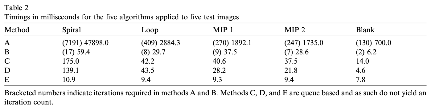
Here, A, B, C and D are the algorithms described by Vincent, with D the most efficient one. E is the priority-queue algorithm by Robinson and Whelan. These experiments clearly show that the priority-queue algorithm is significantly more efficient. The reasoning also makes sense: the priority queue ensures that each pixel gets updated only once, whereas the FIFO queue potentially updates some pixels many times. And so this is the algorithm that I implemented in DIPlib many years ago.

About two months ago, I was replacing an old, no longer supported mathematical morphology library (used in some code I maintain at work) with DIPlib. To do so, I compared each function in the old library with the equivalent DIPlib function to make sure the results were identical. At the same time I compared running times. Some functions were a bit faster in one library, some a bit faster in the other, and some, like basic dilations with larger structuring elements, were significantly faster in DIPlib. Of course, I took the opportunity to improve the implementation of some of these functions that were a little slower in DIPlib, where obvious gains could be made. But the morphological reconstruction function really surprised me. The old library’s implementation was ten times faster than DIPlib’s!

Examining the DIPlib implementation, I noticed that I had been lazy when making the original implementation. Marking border pixels in a flag image allows the algorithm to skip testing coordinates before accessing neighbors for most pixels in the image, speeding up processing by about 20%. Ensuring consistent strides so that the same offsets can be used in the f, g and intermediate flag images sped up processing by another 20%. And a few small things here and there rounded out improvements to a total of about 50%. But this meant that the implementation was still five times slower than that in the old library.

So I took a look at the code in the old library, and found that it implemented the algorithm proposed by Vincent (method D in the table above), which was supposed to be anywhere from two times to 14 times slower than the priority queue algorithm.

I was doing my timing comparison on quite a large image. Robinson and Whelan did their experiments on quite small images, a much larger fraction of which would have fit in their cache. And a priority-queue algorithm processes pixels in the image in a rather disorganized way. Putting these points together, it becomes obvious that I was seeing a cache miss for just about every pixel processed, whereas Robinson and Whelan were seeing a lot fewer cache misses, and my cache misses were likely more expensive too. I believe that this is why I was seeing such slow execution in the DIPlib implementation. In contrast, Vincent’s algorithm uses a raster scan and an anti-raster scan to do a large chunk of the propagation. These scans are very cache-friendly.

So I rewrote the DIPlib implementation to be a combination of the two algorithms: it first applies a raster scan and an anti-raster scan to do a large chunk of the work. The second scan, in anti-raster order, also initializes a priority queue, enqueueing all pixels from which it is possible to propagate right and down (since this scan is propagating left and up). Next, the algorithm processes the pixels in the priority queue, enqueuing neighbors from which further propagation is possible, until the queue is empty. Each pixel is thus updated no more than three times. This implementation was, in my tests, a bit faster than Vincent’s, which uses a FIFO queue and therefore each pixel can potentially be updated many times.

So, lessons learned:

1. One cannot make assumptions about which algorithm or implementation is faster without actually measuring times.
2. Timings from 15 years ago are likely no longer relevant.
3. Sometimes it’s good to take another look at older, superseded algorithms.
4. What is true for small data is not necessarily true for large data.