Cris’ Image Analysis Blog

First of all: Happy New Year!

Over the holidays I’ve been learning about dithering, the process of creating the illusion of many grey levels using only black and white dots. This is used when displaying an image on a device with fewer than the 64 or so grey levels that we can distinguish, such as an ink-jet printer (which prints small, solid dots), and also when quantizing an image to use a colour map (remember the EGA and VGA computer displays?). It turns out that this is still an active research field. I ran into the paper Structure-aware error diffusion, ACM Transactions on Graphics 28(5), 2009, which improves upon a method presented a year earlier, which in turn improved on the state of the art by placing dots to optimize the appearance of thin lines. This got me interested in the basic algorithms, which I had never studied before. Hopefully this post will give an understanding of dithering and its history.

(As always, the code in this post is for MATLAB, and some of it requires DIPimage.)

Random dithering

The reason one needs dithering is quite obvious. If your display can only display black and white pixels, a grey-value image like this:

img = [newim(150,64)+1;newim(150,64)+64;newim(150,64)+85;newim(150,64)+127];
img = [readim('trui'),img,xx('corner')]

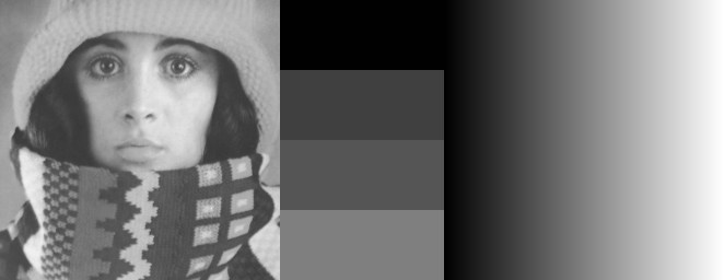
will end up looking like this:

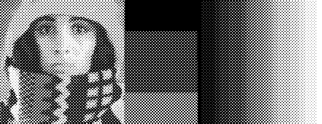
out = 255*(img > 127)

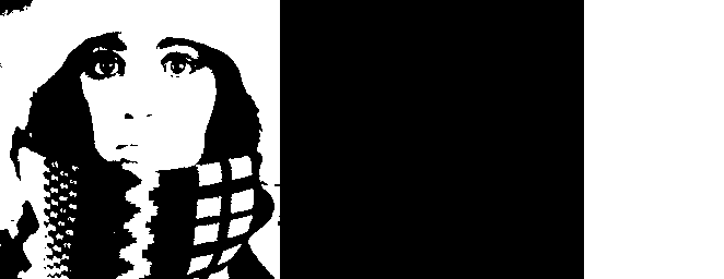
Obviously, more is lost than necessary. What we want to do is put 50% of pixels to on in a middle-grey (127) region, 25% of pixels to on in a region of grey value 63, etc. The simplest way to accomplish this is using a random process, in which a pixel of value 127 has a 50% chance of becoming white, a pixel of value 63 has a 25% chance, etc. This two lines of code accomplishes this:

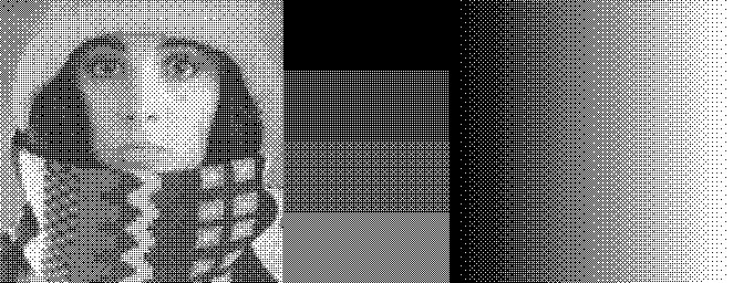
t = noise(newim(img),'uniform',0,255);
out = 255*(img > t)

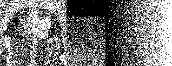
We simply replaced the constant threshold value of 127 with a random one, in the range 0 to 255. The problem with this output is that it looks noisy! We basically added white noise to the image, which has equal power at high and low frequencies. The goal is to avoid changing the low frequencies, so that, when viewed from an appropriate distance, the image looks identical to the original (the further away from the display you are, the more high-frequency components get lost). Thus, we want a high-frequency noise with no power at lower frequencies. Such noise is called blue noise, and can be generated simply by removing the low-frequency components of the noise image t:

t = hist_equalize(t-gaussf(t,2))*(254/255);
out = 255*(img > t)

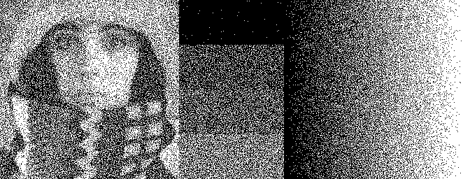
Note that I used hist_equalize to make sure that the values in the image t are uniformly distributed. The result is still noisy, of course, but much more detail of the original image is preserved. This is because the low-frequency components of the image are not disturbed as much. I urge you to look at the Fourier transform of these various images and compare what happens at low and high frequencies in each.

Halftoning

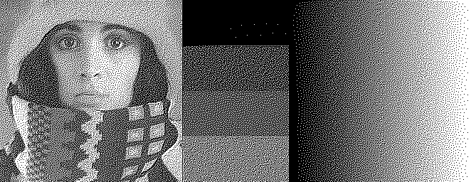
Artists have been using techniques similar to dithering for many centuries: wood, leather or metal plates were etched, then inked and pressed against paper to produce a black and white impression. By creating small structures, the artists could create the impression of different levels of grey. With the advent of photography, an optical technique to create such an etching from a photograph was developed. This technique, halftoning, allowed photographs to be printed with ink on paper, for use in books and newspapers. In brief, the method involved projecting the image through a screen composed of tiny dots (such as a silk cloth). Brighter parts of the image will produce larger dots on the screen than darker parts. A photochemical process etches the dots into the metal plate. Nowadays this is done digitally, and at much higher resolution, but newspapers still use variable-sized dots to reproduce photographs.

Halftoning can be implemented in a quick-and-dirty way thus:

s = 2;
t = (cos((pi/3/s)*(xx(img)+0.2))*cos((pi/3/s)*(yy(img)+0.3))+1)*127;
out = 255*(gaussf(img,s) > t)

But please note, this is not the way it should be done!

I created a mask for thresholding that, similarly to earlier masks, is uniformly distributed in the range 0 to 255. However, the points now are ordered, so that the “on” pixels in a grey area are clustered together. The parameter s determines the size of the dots, and I’ve smoothed the image before thresholding so that the dots look more like dots (it’s not really necessary to do the smoothing). Because we have an ordered mask now, there is a limited number of grey values. Our dots grow with whole pixel increments. When reducing the size of the dots, the number of reproducible grey values is also reduced:

s = 1;
t = (cos((pi/3/s)*(xx(img)+0.2))*cos((pi/3/s)*(yy(img)+0.3))+1)*127;
out = 255*(gaussf(img,s) > t)

Ordered dithering

The quick-and-dirty halftoning I implemented above is a form of ordered dithering. The randomness of the noise mask is replaced by a fixed, repeated pattern. However, clustering the “on” pixels in this way creates strong artefacts (the dots!) that are not necessary for electronic displays. A printer benefits from the clustering because it becomes easier to control the amount of ink on the paper (ink tends to diffuse into the paper, for example). But for your computer’s screen a more pleasant effect is achieved when the “on” pixels are distributed as evenly as possible. Bayer (1973) descried a mask to be used for this purpose:

m = [
    1 , 49 , 13 , 61 ,  4 , 52 , 16 , 64
   33 , 17 , 45 , 29 , 36 , 20 , 48 , 32
    9 , 57 ,  5 , 53 , 12 , 60 ,  8 , 56
   41 , 25 , 37 , 21 , 44 , 28 , 40 , 24
    3 , 51 , 15 , 63 ,  2 , 50 , 14 , 62
   35 , 19 , 47 , 31 , 34 , 18 , 46 , 30
   11 , 59 ,  7 , 55 , 10 , 58 ,  6 , 54
   43 , 27 , 39 , 23 , 42 , 26 , 38 , 22 ] * (255/65);

The mask contains 64 different values, thus it is possible to threshold the image at 64 different grey levels, producing a different pattern for each of 65 different grey levels. It is possible to use smaller subsets of this mask, such as [1,4;3,2], for 5 different grey levels. This pattern is repeated to create a mask of the same size as the image, then we threshold as before:

sz = size(img);
t = repmat(dip_image(m),ceil(sz/n));
t = t(0:sz(1)-1,0:sz(2)-1);
out = 255*(img > t)

This method is most commonly used in computer displays with limited palettes, because it is simple, fast, and deterministic (meaning it can be used in animations). Also, this is the best method to render large areas of uniform intensity, such as in GUIs. But for a photograph it leaves quite a bit to be desired. This is where error diffusion comes in.

Error diffusion dithering

In 1975, Floyd and Steinberg introduced error diffusion, a process where the error made at one pixel, when it is assigned a 0 or a 255, is passed on to its neighbours. Much like a real diffusion process, the error is spread so that it can be compensated for later on. The image is scanned row by row once. Each pixel visited is assigned a value, and the difference between that value and the input value is split among the neighbours not yet visited:

out = double(img);
sz = size(out);
for ii=1:sz(1)
   for jj=1:sz(2)
      old = out(ii,jj);
      new = 255*(old >= 128);
      out(ii,jj) = new;
      err = new-old;
         if jj<sz(2)
            % right
            out(ii  ,jj+1) = out(ii  ,jj+1)-err*(7/16);
         end
      if ii<sz(1)
         if jj<sz(2)
            % right-down
            out(ii+1,jj+1) = out(ii+1,jj+1)-err*(1/16);
         end
            % down
            out(ii+1,jj  ) = out(ii+1,jj  )-err*(5/16);
         if jj>1
            % left-down
            out(ii+1,jj-1) = out(ii+1,jj-1)-err*(3/16);
         end
      end
   end
end
out = dip_image(out)

This scheme produces a pseudo-random pattern, somewhere in between the fully random and fully ordered patterns we have seen so far.

It is a very, very simple algorithm, the code is only slightly complicated by the checking for out-of-bounds writes, and could be simplified by adding a dummy border to the image. Note, however, several structured patterns appearing at specific grey values (best visible in the ramp on the right side of the image). The four uniform blocks also show problems. These specific grey values are known to cause these problems, and is why I included them in the test image. A regular pattern is produced, but broken at some locations. These breaks produce visual artefacts that were not present in the input image. A third problem is that, sometimes, dots will be placed in little diagonal lines. These are called worms and significantly affect the visual quality of the output. Again, look at the Fourier transform of this image; you’ll notice some strong peaks at middle and high frequencies, caused by these artefacts.

Since this algorithm was published, many publications suggested improvements to the basic scheme: larger windows over which to diffuse the error, different weights to the diffusion kernel, changing the traversal direction on even and odd lines, etc. etc. The most simple and effective one is to add a little bit of randomness to the process, though this is unsuitable for some purposes. In the code above, change the threshold code to read:

      % new = 255*(old >= 128);
      new = 255*(old >= 128+(rand-0.5)*100);

In 2001, Ostromoukhov proposed to change the diffusion coefficients depending on the input grey level. They determined “difficult” grey levels experimentally, and chose weights for them that optimize certain criterion in the output of a uniform image with that grey level (for those interested: they aimed at making the spectrum of the error image most similar to blue noise as possible). Weights for other grey levels were determined through linear interpolation. Thus, this algorithm is as fast as the original error diffusion, but with much better results. Zhou and Fang extended the Ostromoukhov algorithm with threshold modulation. The threshold they used also depends on the input grey level, and is determined experimentally for a set of key grey values and interpolated linearly for other grey values. The code below implements this Zhou-Fang dithering, which includes also the alternating left-right, right-left processing of rows. Again, if we were to add a dummy border to the image, the code would be a bit simpler.

coef = [ % [ index, right, left-down, down ]
     0,      13,      0,      5
     1, 1300249,      0, 499250
     2,  214114,    287,  99357
     3,  351854,      0, 199965
     4,  801100,      0, 490999
    10,  704075, 297466, 303694
    22,   46613,  31917,  21469
    32,   47482,  30617,  21900
    44,   43024,  42131,  14826
    64,   36411,  43219,  20369
    72,   38477,  53843,   7678
    77,   40503,  51547,   7948
    85,   35865,  34108,  30026
    95,   34117,  36899,  28983
   102,   35464,  35049,  29485
   107,   16477,  18810,  14712
   112,   33360,  37954,  28685
   127,   35269,  36066,  28664];
x = coef(:,1);
y = coef(:,2:4);
y = bsxfun(@rdivide,y,sum(y,2));
coef = [interp1(x,y(:,1),0:127)',interp1(x,y(:,2),0:127)',interp1(x,y(:,3),0:127)'];
coef = [coef;flipud(coef)];
strg = [
     0, 0.00
    44, 0.34
    64, 0.50
    85, 1.00
    95, 0.17
   102, 0.50
   107, 0.70
   112, 0.79
   127, 1.00];
strg = interp1(strg(:,1),strg(:,2),0:127)';
strg = [strg;flipud(strg)];
img = double(img);
out = img;
sz = size(out);
for ii=1:2:sz(1)
   for jj=1:sz(2)
      old = out(ii,jj);
      new = 255*(old >= 128+(rand*128)*strg(img(ii,jj)+1));
      out(ii,jj) = new;
      err = new-old;
      weights = coef(img(ii,jj)+1,:); % +1 to account for MATLAB indexing into table
         if jj<sz(2)
            % right
            out(ii  ,jj+1) = out(ii  ,jj+1)-err*weights(1);
         end
      if ii<sz(1)
            % down
            out(ii+1,jj  ) = out(ii+1,jj  )-err*weights(3);
         if jj>1
            % left-down
            out(ii+1,jj-1) = out(ii+1,jj-1)-err*weights(2);
         end
      end
   end
   ii = ii+1; % even rows go right to left
   for jj=sz(2):-1:1
      old = out(ii,jj);
      new = 255*(old >= 128+(rand*128)*strg(img(ii,jj)+1));
      out(ii,jj) = new;
      err = new-old;
      weights = coef(img(ii,jj)+1,:); % +1 to account for MATLAB indexing into table
         if jj>1
            % right
            out(ii  ,jj-1) = out(ii  ,jj-1)-err*weights(1);
         end
      if ii<sz(1)
            % down
            out(ii+1,jj  ) = out(ii+1,jj  )-err*weights(3);
         if jj<sz(2)
            % left-down
            out(ii+1,jj+1) = out(ii+1,jj+1)-err*weights(2);
         end
      end
   end
end
out = dip_image(out)

Iterative dithering

I think this is as good as simple error diffusion can possibly be. More complex algorithms use an iterative approach, where dots are placed to minimize some error criterion. These algorithms are typically several orders of magnitude slower than error diffusion, and, of course, the most difficult thing about them is to design a correct error measure. As I mentioned at the beginning of this post, a recent paper took the improvements of an iterative algorithm, designed to optimize dot placement for preserving thin lines (“structure-aware dithering”), and developed an error-diffusion scheme with similar results. It uses even larger lookup tables than the Zhou-Fang scheme (about 1.3 Mb of them), together with frequency and orientation analysis of local neighbourhoods, to determine error diffusion weights and threshold modulation weights. The paper shows some fantastic results, but this method is way too complex for one blog post! The paper comes with the source code in the supplementary material, which I compiled and ran on my test image:

Doing all the analysis takes several seconds on this small image, meaning that the whole process takes several seconds instead of being instantaneous. But then again, a few years down the road this will be instantaneous as well.