Cris’ Image Analysis Blog

I sometimes find people confuse the Hessian and the Structure Tensor. This post will hopefully help disambiguate them.

In 2D, the Hessian of an image is defined as

The Structure tensor is defined as

Though the two written equatinos look fairly similar, the computations these equations represent are not that similar, and the properties of these tensor images are not either.

The Hessian

The Hessian matrix is formed by the second order partial derivatives,

To compute partial derivatives, we’d of course choose Gaussian derivatives (see also here and here for more on Gaussian filtering). When applied to an image, we’d obtain a matrix with all three (in 2D) second order derivative images. In DIPlib (and DIPimage) we can represent this as a tensor image, and image where each pixel has a tensor value. The function Hessian computes this image:

import diplib as dip

img = dip.ImageRead('examples/erika.tif')
H = dip.Hessian(img)
dip.TileTensorElements(H).Show()

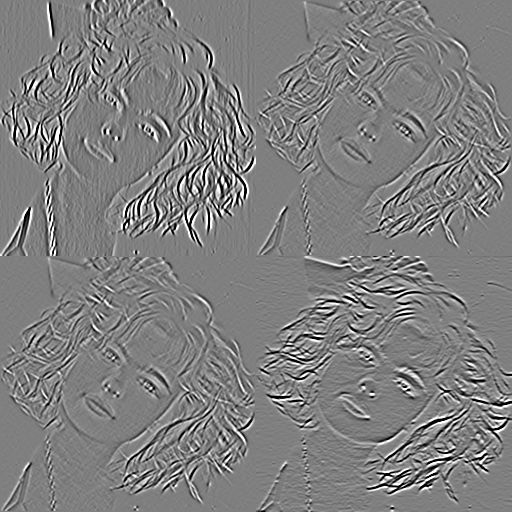
Note that the notation is useful because it provides a compact notation that is dimensionality-independent, and explains how the matrix is extended from 2D to higher dimensionalities. However, we don’t compute it by applying two first-order partial derivatives in sequence. Instead, we compute the second-order derivatives directly. This is more efficient. Also, since this is a symmetric matrix, DIPlib computes and stores the off-diagonal component only once.

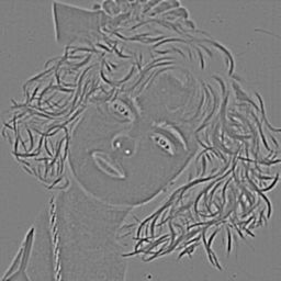
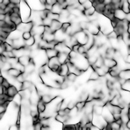
The trace of the Hessian (the sum of the diagonal) is the Laplacian:

dip.Trace(H).Show()

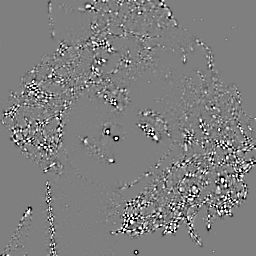
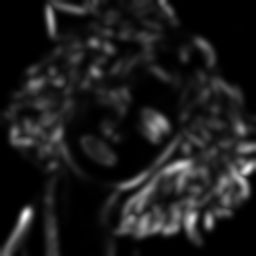
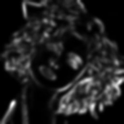
The determinant of the Hessian () can be used to distinguish extrema from saddle points. It is therefore useful to identify useful features to track, or important points in the image that can be matched. The determinant of the Hessian is the basis of the SURF detector [1], though SURF uses some rough approximation to derivatives using box filters.

dip.Determinant(H).Show()

The Structure Tensor

The Structure Tensor is the outer product of the gradient vector with itself, locally averaged. It is thus formed exclusively by first-order partial derivatives, not second-order ones as in the Hessian.

where indicates the partial derivative along axis x. The overlines indicate averaging. The Structure Tensor is typically computed by averaging within a given window, and more often than not you’ll see a Gaussian window being used because of its unique properties.

Thus, the Structure Tensor can be computed as follows:

g = dip.Gradient(img)
# S = g * dip.Transpose(g)  # For versions prior to DIPlib 3.3.0
S = g @ dip.Transpose(g)    # For DIPlib 3.3.0 and later
S = dip.Gauss(S, 3)

dip.TileTensorElements(S).Show()

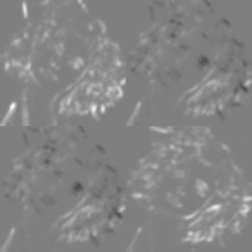
When multiplying the vector image g with its own transpose, DIPlib outputs a symmetric matrix image, where the duplicated elements are not computed and not stored. So, just like the Hessian image H, S only stores three values per pixel.

DIPlib has a function that does the three steps above for you:

S = dip.StructureTensor(img, tensorSigmas=3)

One can think of the outer product of the gradient vector with itself as a mapping that allows local averaging without loss of relevant information. For example, think of a line. The gradient is always perpendicular to the line, but on one side it points one way, and on the other side it points in the opposite direction. These two vectors have opposite direction, but the same orientation.

Local averaging would have these opposite vectors cancel out, whereas we would like to average their orientation, so as to determine the line’s orientation. A common trick around this is to double the angles, such that angles 180 degrees apart become the same. But then vectors 90 degrees apart will cancel out. So just a mapping of the angle to another angle will not allow us to preserve all information. Similarly, any mapping of 2D vectors to other 2D vectors will not allow us to preserve all information. We need to map the 2D vectors to a higher-dimensional space. The Structure Tensor maps the 2D vectors to a 3D space (there are four components, but two of those are identical).

A friend of mine, back in our days as a PhD student, referred to this mapping as the “french fry bag mapping”, but you’d have to be Dutch to get that reference. For an international audience, let’s call it the “cone mapping”. Imagine you have a sheet of paper. From a point in the middle you draw two vectors in opposite direction. After making a cut from that middle point to an edge, you can twist the paper such that the two vectors overlap. The sheet of paper is now a cone. We’ve mapped the two 2D vectors to the same 3D vector. A third vector that was perpendicular when the paper was flat will now point to another place in the 3D space. Averaging these 3D vectors together will not have them cancel out, instead producing a vector pointing straight up. The average preserves the average strength of the input vectors, their average orientation, and how strongly their orientations differed.

To retrieve the information stored in the Structure Tensor, an eigenvalue analysis is typically applied. For each pixel we thus obtain two eigenvalues, and an eigenvector’s orientation (the other eigenvector is perpendicular to the first, and thus redundant).

E, V = dip.EigenDecomposition(S)
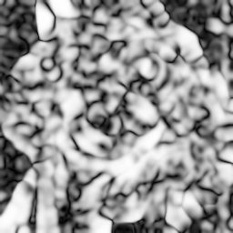
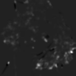
E(0).Show()
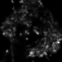
E(1).Show()
dip.Angle(V(slice(0,1))).Show('orientation')

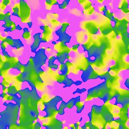
The eigenvector encodes the orientation of the line, the two eigenvalues encode the gradient strength (energy) and variation (isotropy). Eigenvalue analysis is typically represented as an ellipse, with an orientation and two axes lengths corresponding to the eigenvalues.

The ellipse in the figure above represents the average (according to the Structure Tensor) of the gradients in a neighborhood. The larger the ellipse, the stronger the gradients in the neighborhood. The more elongated the ellipse, the more uniform are the edge orientations within the neighborhood. Conversely, the more circular the ellipse, the more varied are the edge orientations.

Thus, if both eigenvalues are similar in magnitude, then the gradients in the local image region point in all directions, the neighborhood is isotropic. If one eigenvalue is much larger than the other, then the gradients in the local image region all point in the same direction (or rather, have the same orientation). There are two common ways to represent this anisotropy measure (with the larger eigenvalue and the smaller one):

The sum of the eigenvalues () is typically used as the energy measure.

anisotropy1 = (E(0) - E(1)) / (E(0) + E(1))
anisotropy2 = 1 - (E(1) / E(0))
energy = E(0) + E(1)

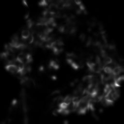
So, for example, points with low anisotropy and high energy would be good points to track:

((1 - anisotropy1) * energy).Show()

If we write this out, we notice that we’re just looking at the smallest eigenvalue:

This is how the Shi-Tomasi corner detector is defined [2].

Because the eigenvalue analysis is rather expensive to compute, Harris and Stephens suggested an approximation computed using the determinant and the trace of the Structure Tensor, , where is typically set to 0.04 [3]. The year before, Noble suggested , which doesn’t require any parameters to tweak [4], but is much less known than Harris’ corner detector.

(dip.Determinant(S) - 0.04 * dip.Trace(S)**2).Show()
(dip.Determinant(S) / dip.Trace(S)).Show()

Conclusion

The Hessian and the Structure Tensor are both similar-looking mathematical expressions that have similar applications, but they have wildly differently computations behind them, and wildly different ways of extracting relevant information. We’ve seen how both of them can be used to detect key points (corners, features to track, etc.). They both can also be used to detect lines (for example the very popular Frangi vesselness measure is based on the Hessian) and many other things. The Structure Tensor is also used in Lucas-Kanade optical flow, and in Weickert’s coherence enhancing diffusion.

This post took a long time to write, but it was fun showing off DIPlib’s tensor expressions (all of the code above would be way more complex to write with OpenCV or scikit-image!), DIPlib’s new Python bindings, any my blog’s new LaTeX-to-SVG capabilities. I hope you got something out of this too.