Cris’ Image Analysis Blog

A frequent problem in image processing is aligning two or more images together. Maybe you have a series of images that partially overlap and need to stitch them into a single, larger image. Maybe you have a video sequence and need to estimate and remove the movement. Maybe you have images of the same subject but in different modalities that you need to combine. In all these cases, the transformation you need to apply to one image to match it to the other is only translation (or shift), rotation, and maybe scaling. (You might also need to apply a correction for lense distortion, but that is outside the scope of this post.)

The most common methods for finding the alignment are all based on markers: First you find a set of distinct points (or markers) in the two images (corners, dots, etc.), then you find the correspondences (figure out which marker in image A corresponds to each marker in image B), then you compute the transformation from those correspondences. And this often works well. The hardest part here is finding the correspondences. When fitting the transformation, some number of mismatches can be accounted for, but most matches need to be correct.

Here I wanted to explain a simpler method to align two images, that is not as widely taught in image processing courses as it should be. It is an efficient, accurate and robust method that directly compares the full images, rather than individual markers. It is based on the cross-correlation, which can be used to find the shift between two images, and the Fourier-Mellin transform, which disregards translation, and converts scaling and rotation to shifts. This method is due to Reddy and Chatterji (1996).

Let’s explore the method step by step, and explain concepts as we go along.

The Fourier Transform

The first step in the method is to compute the magnitude of the Fourier Transform (FT). We’re actually computing the Discrete Fourier Transform (DFT), which is distinct but strongly related to the Fourier Transform, which is defined in the continuous domain. The DFT is computed efficiently using the Fast Fourier Transform algorithm (FFT). But we’ll refer to it simply as the FT.

I’ll assume we all know what the FT is, but I’ll summarize really quickly here: The FT is a reversible transformation of the image that is useful to study linear systems. The FT maps a complex-valued function to another complex-valued function. Complex values can be interpreted as having a real and an imaginary component, or, equivalently, a magnitude and a phase.

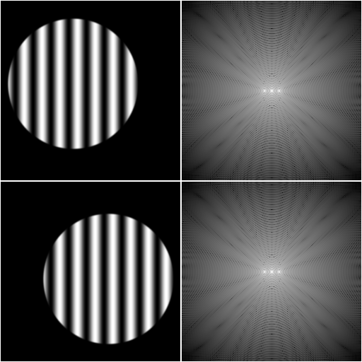
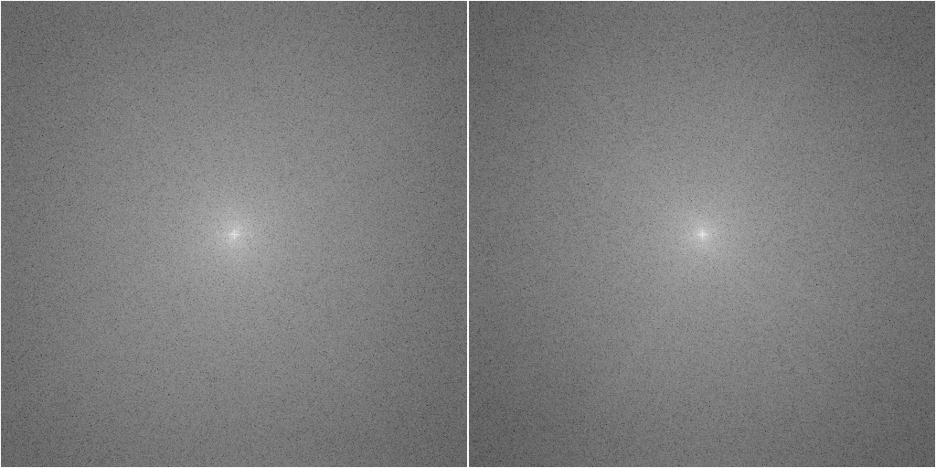
A shift in the image is encoded solely in the phase of the FT (images on the right are the magnitude of the FT of the images on their left):

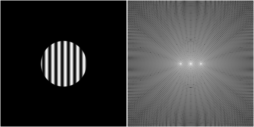
So, taking the magnitude of the FT, we’ve removed the shift from the problem. But what happened to the scaling and the rotation? A scaling of the image results in an inverse scaling of the FT:

And a rotation of the image results in an equal rotation of the FT:

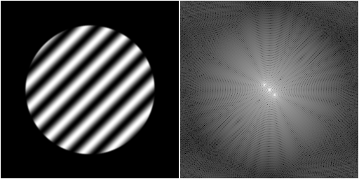
However, because the input image was real-valued, the FT is symmetric about the origin, and therefore we conflated the rotation with φ and the rotation with φ+π. We are no longer able to distinguish a rotation of 180°.

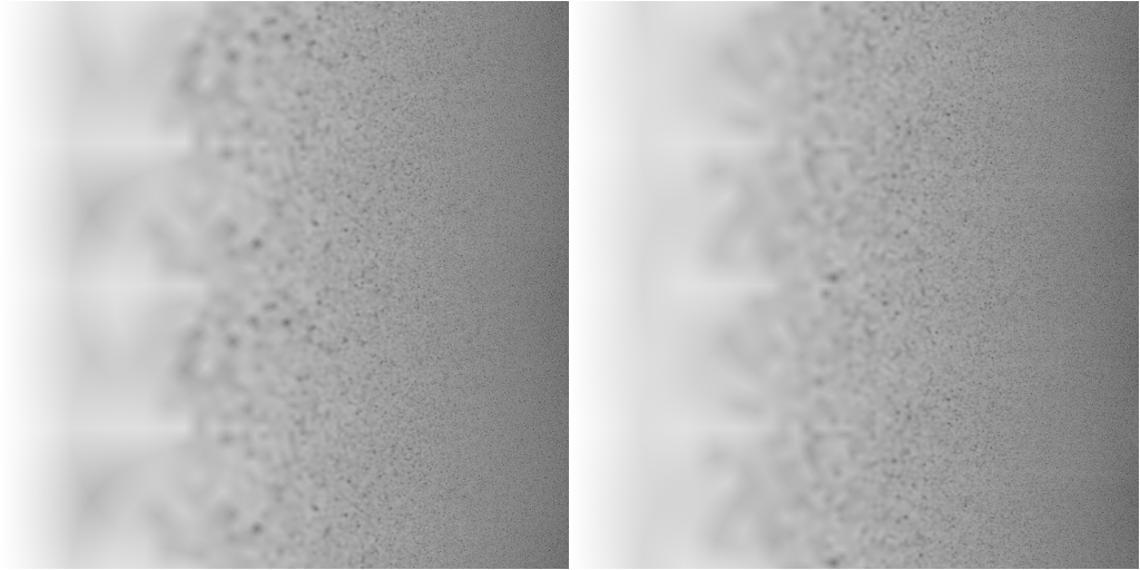
After this first transformation, we have simplified the problem of estimating shift, rotation and scaling to a problem of estimating only rotation and scaling. Next, we apply a log-polar mapping. This is a mapping where the image is deformed in a particular way, resulting in the x-axis of the output being the logarithm of the distance to the center of the input image, and the y-axis being the angle around this center:

A rotation around the center of the image corresponds to a vertical shift of the log-polar mapped image. And a scaling will correspond to a horizontal shift of the log-polar mapped image. We thus have converted the rotation and scaling to a simple translation. This is the Mellin transform part of the Fourier-Mellin transform.

Cross-Correlation

Finding a shift between two images is fairly straight-forward using the cross-correlation. In short, we multiply the two images together and compute the sum of the result, yielding a single value. We do this for every possible shift of one image w.r.t. the other. This can be computed efficiently using the FFT. The shift for which the cross-correlation function is largest is the shift that makes the two images most similar. By fitting a parabola to the 3×3 neighborhood of the pixel with the largest value, we can determine its location with sub-pixel precision.

There are different ways to normalize the cross-correlation to increase the sharpness of the peak, and thus improve the localization accuracy. To learn more about these normalization methods, see the DIPlib documentation for dip::CrossCorrelationFT()

Once we found the shift in the log-polar mapped FT image, we can calculate the rotation and scaling for the one image to match the other. Except that we still need to disambiguate the 180° rotation!

What about the shift?

So now we can transform one of the two images to match the other with only a shift and a possible 180° rotation left. We can compute this partially-aligned image, then use the cross-correlation again to find this missing shift. We can apply this cross-correlation twice: once with the transformed image, and once with the transformed image rotated by 180°. One of these two will yield a higher cross-correlation peak, because it will match the other image better.

Example

An example will make all of the above more clear. I’ll be using DIPlib in Python.

Let’s say we have these two input images, img_a and img_b:

import diplib as dip
import numpy as np

img_a = dip.ImageRead("image A")
img_b = dip.ImageRead("image B")

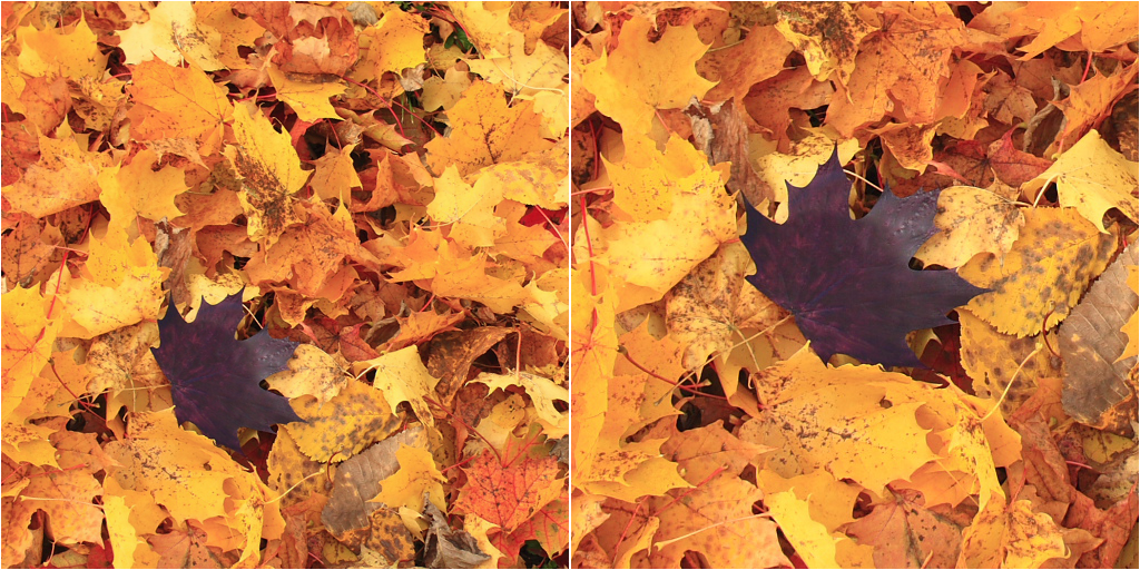
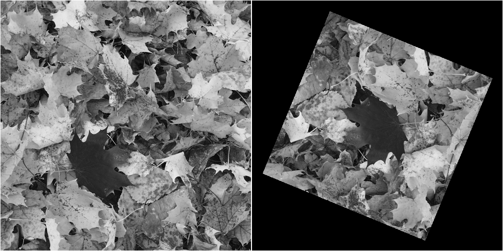
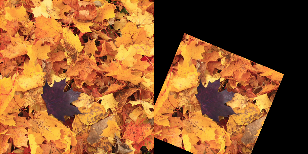
img_b (right) is a crop of some original image. img_a (left) is a different crop obtained after rotating the original image clockwise by π/8 radian and scaling it by a factor of 0.7.

For simplicity, we’ll consider only the green channel, which has good contrast across the image:

gray_a = img_a(1)
gray_b = img_b(1)

We can apply the method to the color images, but we won’t gain anything. After finding the transformation needed to align the gray-scale images, we can apply that transformation to the color image.

We’ll start by computing the FTs of the two images, after applying a windowing function. We discard the phase, and apply a log mapping to improve local contrast:

ft_a = dip.FourierTransform(dip.ApplyWindow(gray_a, "GaussianTukey", 10))
ft_b = dip.FourierTransform(dip.ApplyWindow(gray_b, "GaussianTukey", 10))
lm_a = dip.Ln(dip.Abs(ft_a))
lm_b = dip.Ln(dip.Abs(ft_b))

The windowing function is important because without it, the FT will be corrupted by the edge effects. Image edges usually show up as a sharp horizontal and vertical line through the origin. These two lines will cause a peak in the cross-correlation at the origin, which will be identical for the two images, giving us a chance to erroneously find a shift of 0.

Note also that dip.FourierTransform() computes the full DFT with the origin in the middle of the output image. When using a different FFT implementation, you’ll need to apply a function such as np.fft.fftshift() to get the origin to be in the middle of the image.

Next, we apply the log-polar transformation to the two images:

lpt_a = dip.LogPolarTransform2D(lm_a, "linear")
lpt_b = dip.LogPolarTransform2D(lm_b, "linear")

The cross-correlation between these two images gives a sharp peak, whose location gives the shift:

find_shift_method = "NCC"  # or "PC" or "CC", depending on which normalization you want to use
shift = dip.FindShift(lpt_a, lpt_b, find_shift_method)
print(f"LPT shift = {shift}")

We get a shift of -32.67 along the x-axis and 224.05 along the y-axis. From that we can calculate the rotation and scaling, simply by inverting the computations applied in the log-polar transform:

maxr = np.min(gray_a.Sizes()) // 2
size = lpt_a.Size(0)
scale = maxr ** (shift[0] / (size - 1))
theta = -shift[1] * 2 * dip.pi / size  # 180 degree ambiguity!
print(f"scale = {scale}, theta = {theta}")

We get a scale of 0.7015 and a rotation of -2.749 radian. We expected a scale of 0.7000, and a rotation of 0.3927 (π/8) radian. -2.749 is π/8 - π, so we are off by exactly 180°. Remember that with the FT, we cannot distinguish between these two rotations. We happen to have found the wrong rotation, but fret not, we’ll fix this soon.

We can apply the scale and rotation to the image, which will leave us with a shifted (and rotated by 180°) version of the final result:

matrix = [scale * np.cos(theta), -scale * np.sin(theta), scale * np.sin(theta), scale * np.cos(theta), 0, 0]
gray_b_transformed = dip.AffineTransform(gray_b, matrix, "linear")

Using this transformed image, we can figure out what shift to apply using cross-correlation again:

cc_method = {
    "CC": "don't normalize",
    "NCC": "normalize",
    "PC": "phase",
}[find_shift_method]
cross = dip.CrossCorrelationFT(gray_a, gray_b_transformed, normalize=cc_method)
loc_1 = dip.SubpixelLocation(cross, dip.MaximumPixel(cross))
print(f"loc_1: coordinates = {loc_1.coordinates}, value = {loc_1.value}")

But because we have two possible rotations, we should compute the cross-correlation with gray_b_transformed and also with that image rotated by 180°. The height of the peak will tell us which of the two rotations is the correct one (a larger cross-correlation result means the images are more similar).

gray_b_transformed.Rotation90(2)
cross = dip.CrossCorrelationFT(gray_a, gray_b_transformed, normalize=cc_method)
loc_2 = dip.SubpixelLocation(cross, dip.MaximumPixel(cross))
print(f"loc_2: coordinates = {loc_2.coordinates}, value = {loc_2.value}")

loc_1 has a value of 0.0261, and loc_2 of 0.2920. It is clear that the rotation used for loc_2 is the better one. The peak for loc_2 is at (197.78, 344.04). The shift we’re looking for is the distance from the origin (the middle of the image) to this peak:

if loc_1.value >= loc_2.value:
    # We use theta as the rotation
    matrix[4] = loc_1.coordinates[0] - cross.Size(0) // 2
    matrix[5] = loc_1.coordinates[1] - cross.Size(1) // 2
else:
    # We use theta + 180 as the rotation
    matrix[4] = loc_2.coordinates[0] - cross.Size(0) // 2
    matrix[5] = loc_2.coordinates[1] - cross.Size(1) // 2
    matrix[0] = -matrix[0]
    matrix[1] = -matrix[1]
    matrix[2] = -matrix[2]
    matrix[3] = -matrix[3]

Using this transformation matrix, we can finally compute the transformed version of img_b that matches img_a:

final = dip.AffineTransform(img_b, matrix, "linear")

This whole process is implemented in DIPlib as dip::FourierMellinMatch2D().