Cris’ Image Analysis Blog

In this post I want to show how easy it is to implement snakes using MATLAB and DIPimage. The next release of DIPimage will have some functionality implementing snakes, and this post is based on code written for that. The first implementation of snakes I made for DIPimage used a custom class, dip_snake, to simplify usage. We decided eventually to do without the class. The code discussed here uses that first implementation, which you can download here [Note: the code in the ZIP file requires DIPimage 2, and is not compatible with DIPimage 3]. The most important bits of the code are identical to that in the next release of DIPimage, but the wrapping is not. Adding the class is a nice excuse to show how to modify DIPimage to understand a new parameter type. I will discuss that in a future post.

Snake theory

A snake (a.k.a. active contour) is a flexible 2D line, which is moved around the image to minimize an energy functional. The line is parametrized by through a variable that goes from 0 to 1. Two functions of this variable, and , define the coordinates of the points along the line. For simplicity, we use the vector . More often than not, the snake is implemented as a closed contour, because it is most often used to segment an object. This is enforced setting .

The energy functional that we want to minimize is defined as:

is an internal energy, meant to force the snake to be small and smooth. It avoids obviously wrong solutions. is an external energy, the one responsible for the snake finding the edges of an object in the image. is therefore defined on the image. A common external energy is the inverse of the gradient magnitude: low energies at the location of the edges, higher energies everywhere else. This energy definition comes from the original paper by Kass, Witkin and Terzopoulos (1988).

Let’s discuss the internal energy first. It is defined as

This looks rather complicated, but it need not be. For starters, and are usually constant (the method has enough parameters as it is, there is no point in making two of the parameters different for every point along the snake!). So what we have left is the magnitude of the first derivative, which is larger for longer snakes, and the magnitude of the second derivative, which is larger for sharper bends. The first part keeps the snake short, the second part keeps it straight. The two parameters, and , define the relative importance of these two terms.

To minimize this energy function we use the Euler-Lagrange equation. After quite some work we end up with the following equation:

(By the way, when you derive this is when you understand why the original definition of the internal energy has that ½ in it!) , the gradient of the external energy, is a force. We call this the external force, , and this is where most of the improvements to snakes were made. I won’t discuss them here.

Solving the equation above is accomplished with the gradient descent method: you convert the snake into a function of time, and replace the 0 with the partial derivative of to time. You can see the reason for this if you assume that, after a long time when the snake has converged to a minimum, it’s derivative to time will be zero, and so the equation above is satisfied.

Next we need to discretize the parameter so we can actually implement this numerically. So we set , with going from 0 to . Because the snake is periodic, , , etc. (Note I’m using the square brackets to denote the discrete indexing, as opposed to the round brackets for continuous-domain functions.) This is also the time when we split the vector into its two components and . The two components of the external force are and . We use the finite difference approximation to the spatial derivatives:

and

This results in the following set of equations:

We can write the whole thing, except the external force, as a -by- matrix :

such that:

Note the simple structure of this matrix. Only 5 diagonals have values in them, the rest of the matrix is 0, no matter how large is. This is called a cyclic pentadiagonal banded matrix, and can easily be inverted using Cholesky decomposition. If the snake were not circular (the two ends not connected) this matrix would be even simpler!

The last step is to discretize the time parameter, adding a step size :

To make this easy to solve, we need to do a little trick: we will assume that the movement of the snake is small enough that the external force doesn’t change much from one time step to the next. We can then substitute in the set of equations above the external force at time , yielding a simple to solve set of equations:

Snake implementation

Finally! We’re ready to start writing code…

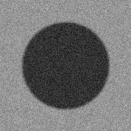
Let’s start with creating an image to test our algorithm on:

img = noise(50+100*gaussf(rr>85,2),'gaussian',20)

We will also need an initial snake to deform:

x = 120+50*cos(0:0.1:2*pi)';
y = 140+60*sin(0:0.1:2*pi)';
hold on, plot([x;x(1)],[y;y(1)],'g')

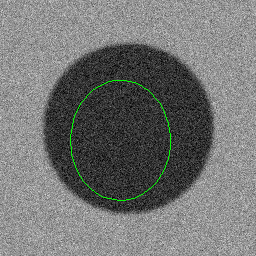
Note that I duplicated the first point at the end when plotting, so that the snake would be a closed contour. I’ll define the parameters now. This is a tricky part, I played around with them until I was satisfied. I haven’t yet seen a clever way of determining these. Because there is no weight for the external force, the parameter needs to be increased if the external force is too weak. To compensate, both and should be decreased by the same factor. Decreasing makes the snake less smooth. Increasing increases the force that wants to shrink the snake; because we started inside the boundary, we want it very small.

alpha = 0.001;
beta = 0.4;
gamma = 100;
iterations = 50;

Next we will compute the matrix inversion. We need to create the matrix and invert it. This is the most complex part of the whole algorithm, but in MATLAB it’s a breeze:

N = length(x);
a = gamma*(2*alpha+6*beta)+1;
b = gamma*(-alpha-4*beta);
c = gamma*beta;
P = diag(repmat(a,1,N));
P = P + diag(repmat(b,1,N-1), 1) + diag(   b, -N+1);
P = P + diag(repmat(b,1,N-1),-1) + diag(   b,  N-1);
P = P + diag(repmat(c,1,N-2), 2) + diag([c,c],-N+2);
P = P + diag(repmat(c,1,N-2),-2) + diag([c,c], N-2);
P = inv(P);

a, b and c are the elements along the 5 diagonals that are not 0. I used the function diag to populate the matrix. inv takes care of selecting an appropriate inversion algorithm. Nothing to worry about here. Note that we need to do this inversion only once, not at every iteration. The matrix is independent of the position of the snake.

Next up is the external force. We need to compute the gradient of the image representing the external energy. This is typically the gradient magnitude. Using DIPimage this is again a breeze! We’ll use gradmag and gradient:

f = gradient(gradmag(img,30));

I’ve used a very large value for the parameter here. This is because the snake starts off far away from the edge we’re looking for, and the external force is the only thing that is able to pull it towards these edges. Many of the improvements to the snake so far have been therefore to increase the “pull” range of edges by modifying the external force. Since I don’t want to go into that, I’ve opted to use a large , which spreads out the gradient over a large area. Another thing to note here is that f is a vector image, that is, each pixel has two values, one for the gradient along the x-axis, and one along the y-axis. f{1} extracts a scalar image containing only the x-component of the gradient, whereas f(100,100) extracts a vector corresponding to the pixel at (100,100).

The last thing to do is to get the value (at sub-pixel locations by interpolation) of the external force at the snake’s control points, and update the position of these control points according to the gradient descent equation we derived. We’ll do this in a loop, iterations times, and plot the resulting snake every 5 iterations. I’m plotting the final result in red:

for ii = 1:iterations
   % Calculate external force
   coords = [x,y];
   fex = get_subpixel(f{1},coords,'linear');
   fey = get_subpixel(f{2},coords,'linear');
   % Move control points
   x = P*(x+gamma*fex);
   y = P*(y+gamma*fey);
   if mod(ii,5)==0
      plot([x;x(1)],[y;y(1)],'b')
   end
end
plot([x;x(1)],[y;y(1)],'r')

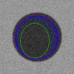
Ok. So now we’ve got a snake, and got it moving towards an edge! Too bad that the snake seems to converge to a point inside the edge. This is because the Gaussian gradient used to compute the external energy had a very large parameter . In a Gaussian smoothed image, edges always move inwards. We could run the loop above again, but using an external force computed with a smaller , since the snake is closer to the edge now. However, there are better alternatives to the external force that do not require this type of multi-scale approach. See for example gradient vector flow or vector field convolution. I won’t go into these, but the next release of DIPimage will have functions to compute these external forces.

Yet another modification to the snake is the so called balloon force. It is an internal force that moves the snake outwards (or inwards if you make it’s weight negative). It can very easily be added to the loop above, as you can see in the function snakeminimize. Go ahead, download and install it into your DIPimage directory [Note: the code in the ZIP file requires DIPimage 2, and is not compatible with DIPimage 3]. There’s a README file with instructions inside. That function uses a class dip_snake, which I will discuss in a future post.