Cris’ Image Analysis Blog

I found an interesting submission on the File Exchange. It uses a very simple set of mathematical morphology filters to find the solution to simple mazes. I have several other solutions, so I decided to write an entry about the subject.

Original solution

This section is paraphrased from File Exchange “Image Analyst“‘s solution. His code uses MATLAB’s image processing toolbox, here we want to use DIPimage, of course.

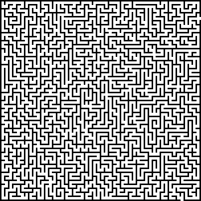
We start by reading in the image with the maze:

inputmaze = readim('maze_solution_01.png')

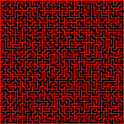
Next we convert it to a grey-value image and threshold it to obtain a binary image. The maze walls are true and shown in red:

maze = colorspace(inputmaze,'grey');
maze = ~threshold(maze)

When we label the binary image, we can clearly see two discrete, separate walls:

maze = label(maze);
dipshow(maze*2,'labels')

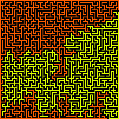
It is fairly easy to see the path from start to finish: it’s the path in between the two colors. To draw this path over the image we can follow this simple sequence of commands, it’s all mathematical morphology. We ignore everything except the first of the two walls:

path = maze==1

Then we dilate the walls by a few pixels, and fill all the holes:

pathwidth = 5;
path = bdilation(path,pathwidth);
path = fillholes(path)

Then we erode by the same amount of pixels and take the difference:

path = path - berosion(path,pathwidth);

The function overlay makes a nice display:

overlay(inputmaze,path)

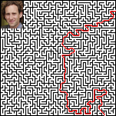
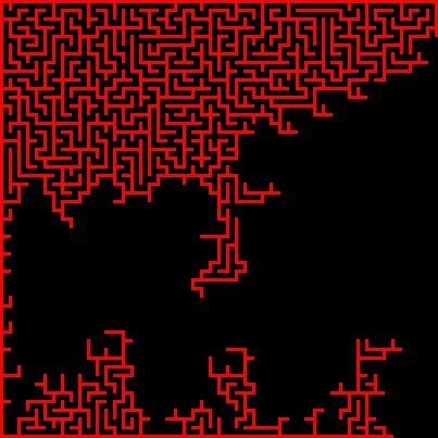
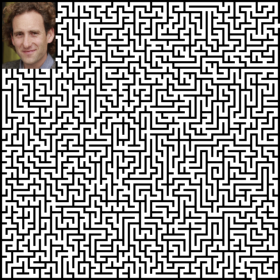
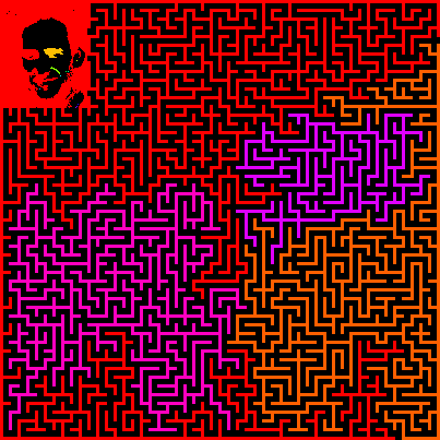
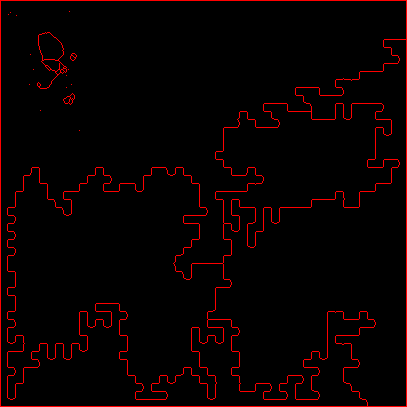
However, when the maze is more complex, things start to go wrong. In this maze I’ve added a photograph, and cut two holes to create more paths:

inputmaze = readim('maze_solution_07.png')

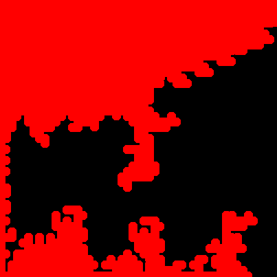
The result after labeling now shows more than two colors:

maze = colorspace(inputmaze,'grey');
maze = ~threshold(maze);
maze = label(maze);
dipshow(maze,'labels')

This is not a big deal, but when we follow the first wall, we’ll find only one of the possible paths, and it’s not necessarily the shortest path. Also, we are lucky that object with ID=1 is a good object to follow. If you pick the wrong object ID here, you’ll end up with a path that doesn’t connect the input and output!

path = maze==1;
pathwidth = 5;
path = bdilation(path,pathwidth);
path = fillholes(path);
path = path - berosion(path,pathwidth);
overlay(inputmaze,path)

Alternate solution

A more robust solution involves using the skeleton. This is a morphological operation that, in rough terms, erodes and object under certain constraints, until the whole object is a single pixel thick. The constraints are that a pixel is never removed if removing it would change the geometry of the object. That is, it will never split an object in two. Let’s go back to the binarised maze image, but now we want the path to be the object, rather than the walls:

inputmaze = readim('maze_solution_07.png');
maze = colorspace(inputmaze,'grey');
maze = threshold(maze);

Because of the way that the skeleton is implemented in DIPimage, we need to add a 2-pixel border around the maze. The skeleton ignores the pixels in this border, so if we don’t add it, part of our maze wouldn’t be taken into account:

maze = extend(maze,imsize(maze)+4);

The skeleton now produces a 1-pixel-thick version of the maze:

path = bskeleton(maze)

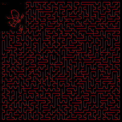
All the dead ends can be easily found, by looking at pixels that have only one neighbor:

deadends = getendpixel(path);
joinchannels('rgb',bdilation(deadends,1,2),path) % fancy display command

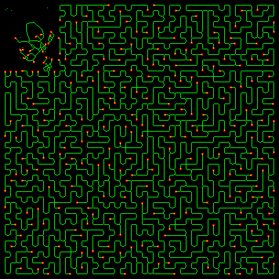
One of the options of the bskeleton function is to remove these dead-end pixels iteratively. This leaves the skeleton as a set of dots and closed loops. By setting the area outside the image to the value 1, we make sure that the bits of the skeleton connected to the image border are kept:

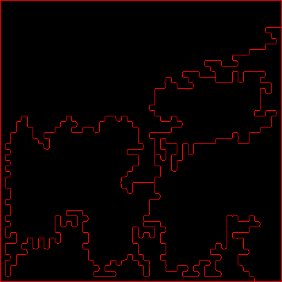
path = bskeleton(maze,1,'looseendsaway')

Notice that there are several loops and dots not connected to the image border. These are caused by the image I added to the maze. We can remove those by keeping only those objects that are connected to the image border:

path = path-brmedgeobjs(path,2)

Finally we’ll remove the temporary image border we added to compute the skeleton, and make the path a little thicker for display:

path = cut(path,imsize(inputmaze));
path = bdilation(path,1);
dipshow(overlay(inputmaze,path,[255,0,0]))

This returned all possible paths from start to finish. But how do we select only the optimal path?

A better solution

The optimal path selection in graph theory is found using Dijkstra’s algorithm. We could easily implement this algorithm by extracting the paths found by the skeleton as a graph. But we want to do this here using image analysis algorithms.

Let’s again start by reading in the maze image and obtaining a binary representation:

inputmaze = readim('maze_solution_07.png');
maze = colorspace(inputmaze,'grey');
maze = ~threshold(maze);

Our first task is to find where the start and stop points are for our path. We’re simply looking for black pixels connected to the image edge:

markers = bpropagation(newim(maze,'bin'),~maze,3,1,1);
markers = label(markers);

Let’s make sure we have exactly two exits, and let’s get their coordinates:

if max(markers)~=2
   error('The maze doesn''t have two exits!');
end
m = measure(markers,[],'center');
start = round(m(1).center)
stop = round(m(2).center)

start =
   401
    37

stop =
   365
   401

The most important step to find the shortest path is the distance transform. This function simply computes the distance from every object pixel in the image to the background. But instead of using Euclidean distances, which take the straight-line distance between the pixel and the background, we use a constrained distance. This constraint forces the distances computed to follow the possible paths through the maze. One of the simplest ways of constraining the distance transform is to weigh the distance with the image’s grey value. That is, the distance between two points is computed as the integral of the grey values along the path between the two points. This is called the grey-weighted distance transform. Incidentally, the grey-weighted distance transform is computed with something very similar to Dijkstra’s algorithm.

By giving the maze walls very high grey values, we can make sure that going around the maze through some long-winded path produces a shorter (weighted) distance than taking a “short-cut” through a wall. We give the maze floors a grey value of 1, so that the distance travelled through the maze is equal to the path length, and the maze walls a value of 10⁶, larger than any path you could possibly draw in such a small image. Furthermore, as with the skeleton, we need to add a little border around the image:

region = extend(markers~=2,imsize(maze)+4); % We compute the distance to the stop point
weights = extend(1+(maze*1e6),imsize(maze)+4);
distance = gdt(region,weights,3);
distance = cut(distance,imsize(maze));
dipshow(distance,[0,2000])

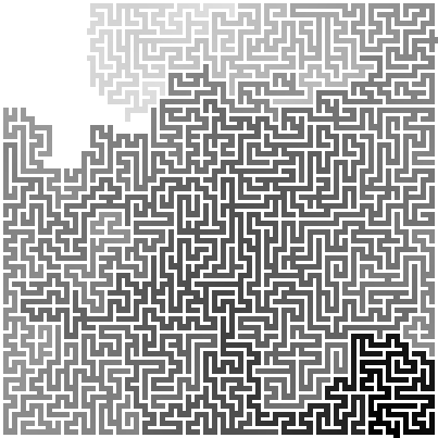
As you can see, the further from the stop point, the higher the grey value of the output is. There is a region in the top-left that cannot be reached at all from the stop point. The distance from start to finish is:

D = double(distance(start(1),start(2)))

D =
   1.0716e+03

To find the path all we now need to do is follow a steepest descent path from the start all the way to the finish. We start at the start point, and look at all its neighbors for the one that has the lowest value. That then becomes the current point and we repeat until we are at the bottom (where distance==0).

current = start;
path = current;
while distance(current(1),current(2))>0
   n = distance(current(1)+[-1,0,1],current(2)+[-1,0,1]);
   [n,step] = min(n);
   step = step-1;
   current = current + step';
   path = [path,current];
end

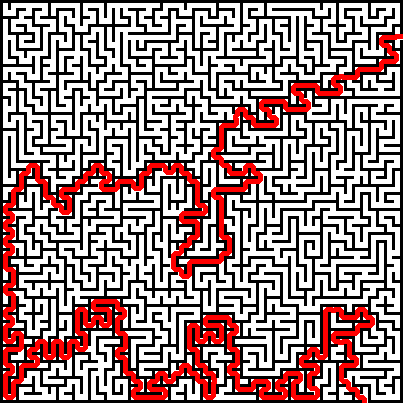
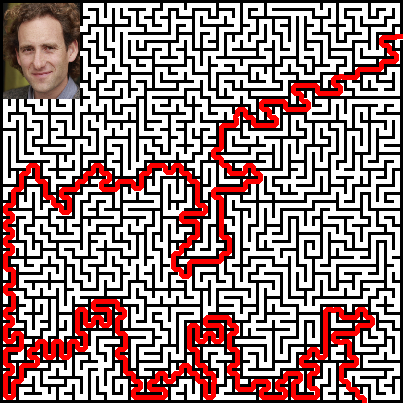
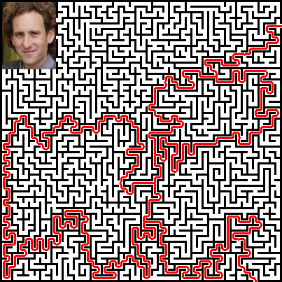
We can now plot the path on the input image:

dipshow(inputmaze)
hold on
plot(path(1,:),path(2,:),'r','linewidth',3)