Panoramic photograph stitching — again
In an earlier post, I described and implemented a method, that was published recently, to stitch together photographs from a panoramic set. In a comment this morning, Panda asked about the parameters that direct the region merging in the watershed that I used. This set me to think about how much region merging the watershed should do. The only limitation that I can think of, is that we need two regions: one touching the left image and one toughing the right. We can easily do this with a seeded watershed: we create two seeds, one at each end of the region where the stitch should be, and run a seeded watershed. This watershed will not create new regions. You should see it as a region growing algorithm, more than a watershed. However, the regions are grown according to the watershed algorithm: low grey values first. That insures that, when the two regions meet, it happens at a line with high grey values (a “ridge” in the grey-value landscape). The graph cut algorithm can now be left out: the region growing algorithm does everything.
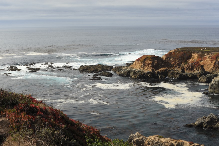
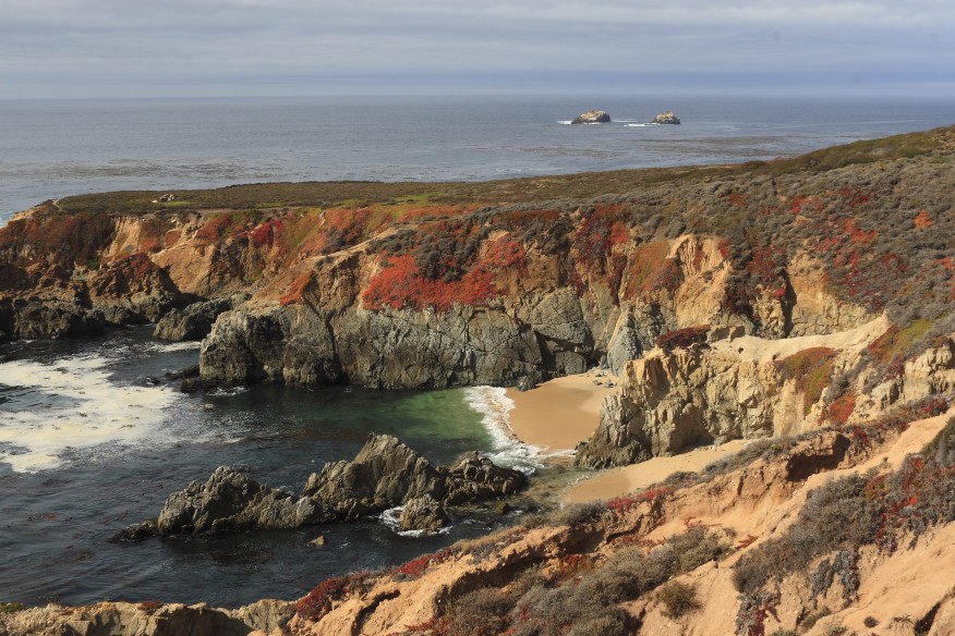
Let’s start with a quick recap. We have two images in variables a
and b
:
I found the coordinates of a common point in the two images, ca
and cb
. Then we extend (and crop) the two images so that they have a common coordinate system:
This is where the two methods start to differ. We again look at the difference between the two images in the stitching region, taking the maximum of the differences in the three colour channels:
d = max(abs(a-b)); d(0:sz(1)-1+s(1),:) = 0; d(sz(1):imsize(d,1)-1,:) = 0;
The only difference with the d
from the earlier blog post is that we do not look at the inverse of the difference, because the region growing algorithm in DIPimage that I will use can grow into high grey values first (i.e. the opposite of what the watershed would do). The next task is to create a seed image. We set the pixels unique to the first image (image a
) to 1, and the pixels unique to the second image to 2. The common region, where the stitch will be, we leave 0, so that the two seeds can grow into this area:
c = newim(d,'sint8'); c(0:sz(1)+s(1),:) = 1; c(sz(1)-1:imsize(d,1)-1,:) = 2;
Now we just run the region growing algorithm:
c = dip_growregions(c,d,[],1,0,'high_first'); w = c==2;
Note that we used the 'high_first'
option. Using 'low_first'
would yield the more traditional seeded watershed. As before, the final composition is trivial using this mask:
out = a; out(w) = b(w);
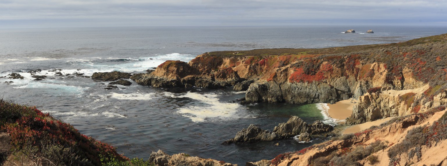
As can be seen below, the two methods choose a different stitching, but both are quite successful. In this example, the region growing method seems better than the graph cut method, but we’d need to do some more extensive testing to know whether this is always the case or not. These two figures show where the images were stitched with each of the two methods, the graph cut method first, the region growing method second:
Finally, a comparison like in the earlier blog post, comparing the blurring, the graph cut, and the region growing methods:
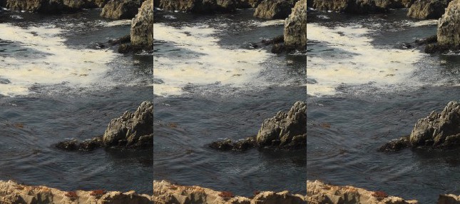
The new method does not duplicate that one rock in the middle of the zoomed area. This might be coincidence, of course. Don’t assume this method is better just because of this one example!
Feel free to download the script I used to generate the images on this page.
Watersheds are minimal graph cuts, in the max norm!
“Some links between min-cuts, optimal spanning forests and watersheds”
Cedric Allene, Jean-Yves Audibert, Michel Couprie, Jean Cousty, Renaud Keriven
Image and Vision Computing (2010)
Thanks Filip!
I was thinking that I should be able to reproduce the watershed result with the graph cut method if I changed the way the weights are calculated…
Hi Cris,
I’ve tried your script. It seems that it will exceeds image boundary since you used a = a(:,0:imsize(a,2)-s(2)-1); Is there any way to solve it? Thanks.
Isabella,
I use DIPimage for the code on this page (and almost everywhere else on this blog). In DIPimage, images have indices starting at 0. You can download DIPimage for free (for non-commercial purposes), look for a link on the right column.
If you do not want to use DIPimage, you’ll have to add 1 to all indexing, and also switch the position of the first two indices (
a = a(1:imsize(a,1)-s(1),:)
).Firstly I would like to thank you for you detailed explanations, but Cris, unfortunately when i am running the above script
I am getting the following erro
Error using dip_image/cat (line 100)
CAT arguments dimensions are not consistent.
Error in dip_image/iterate (line 89)
a(jj) = feval(fun,args{:});
Error in panor (line 92)
stitch = iterate(‘cat’,1,stitch2,stitch3,stitch4);
Could you please help me to debug this. Thanks
Hi prashanth,
I’m not sure why you get this error, the script works well for me. Make sure
imsize(stitch2)
returns the same image size asimsize(stitch3)
andimsize(stitch4)
. In any case, this line just puts 3 different outputs together to display them side-by-side on the web page; it is not a part of the stitching algorithm.Hi Cris,
% Alternative: the composition I made in the original blog post
out = readim(‘bigsur.jpg’);
stitch3 = out(sz(1)+s(1):sz(1)-1,:);
I get error “”bigsur.jpg” not found.”
and when I make this ‘bigsur1.jpg’ or ‘bigsur2.jpg’, I get the same error as prashanth got above,
??? Error using ==> dip_image.cat at 100
CAT arguments dimensions are not consistent.
Error in ==> dip_image.iterate at 89
a(jj) = feval(fun,args{:});
Error in ==> bigsur_new at 92
stitch = iterate(‘cat’,1,stitch2,stitch3,stitch4);
please help me to sort it out.
Hi Ramzan,
The file ‘bigsur.jpg’ is the stitched result from the first post on panoramic stitching that I wrote (linked in the beginning of this post). If you use that image, the dimensions for the three little images should match and the ‘cat’ command should work fine. But as I said to Prashanth above, this part of the script is only to make the image comparing the three stitching methods, it is not necessary at all for stitching.
Dear Cris, a bundle of thanks for helping me out. Everything is fine now. I am novice to Matlab and image stitching but I have learned a lot from your code. My sincere salute to you, People like you are great asset to the learner like me.
Hi Cris, I run the code of region growing, it’s fast, and the results are good for many images of my task. but I need to coding the region growing algorithm by c. If you could tell me the paper’s name the function dip_growregions based on, or some other advice. thanks.
Liming,
The
dip_growregions()
function simply implements the seeded watershed, but by using the'high_first'
option, the ordering of the pixels is inverted. I implemented this in two steps: First I go over the whole image and find all foreground pixels (pixels with value different from zero) that have a background neighbour (value 0). I put these pixels in a priority queue, where the priority value is the grey value of that pixel in the second input image. In the second step, I take pixels out of the priority queue, highest priority first, and examine all its neighbours. Neighbour pixels that are background I set to the value of the pixel I took out of the priority queue, and add to the priority queue. When the queue is empty, all pixels in the image will have a value different from 0. There are other ways of implementing the seeded watershed, you can find these algorithms in the literature.Good luck!
Firstly I would like to thank you for you detailed explanations,
i want to know can i use this algorithm for stitching video in real time video player ?
if yes , how i can do this plz. ? can you help me ?
Rami,
I think this algorithm is quite slow. But it might be possible to create a real-time implementation, who knows? Give it a try and let us know if it is possible or not!
Hi Cris,
I want to say a thanks for your sharing this smart idea!
Two points:
1. the crop code needs to be updated also:
a = a(:, 0:imsize(a, 2) + s(2) – 1);
b = b(:, 0:imsize(b, 2) + s(2) – 1);
2. How you generate the red stitched lines?
panovr,
Good point, thanks! I’ve fixed the script here too.
The red stitch line I probably generated with something like this:
Where the
[255,0,0]
is the colour of the line.Hi Cris,
thanks for the tip!
I just thought another question: now that we have two methods for image blending, how can we evaluate these two methods, which one is better? If we evaluate the results by our eye, this is subjective. How about objective evaluation?
panovr,
That is a very good question, but I don’t know the answer.
The image blending in this case is done for making a pretty picture, so the only valid (IMO) evaluation is a subjective one. You’d have to find test subjects that compare pictures two by two, and pick the ‘prettiest’ in each case. Then you see which method is chosen more often, and if this difference is significant or not.
If the blending were done for other reasons, you’d have to see which method is better by evaluating how well you can accomplish the task you intend to do with the blended images. For example, if it is for quantitative microscopy, you’d see which of the blending methods gives you the best quantification. In this scenario, the differences are likely to not be significant, this is why not much effort is typically put into blending microscope images (AFAIK).
Hi Cris,
my evaluation aim is to compare the two methods which can generate a more “seamless” blending image.
I will do experiment on more data sets.
By the way, I’m reading DIPlib and DIPimage documents, what the meaning of “scalar image” in the doc?
panovr,
A scalar is a single value. A scalar image has one value per pixel (i.e. it is a grey-value image). DIPimage also supports vector and tensor images, and hence the use of the term “scalar” in this context.
Let me know the results of your experiments!
Hi Cris,
how about color image, for example, RGB or RGBA image? Color image has 3 values (red, green and blue) or 4 values (red, green, blue and alpha) per pixel. Is this vector image as your note?
I’m starting to do the experiments, and I have sent an email to you to describe my evaluating process.
panovr,
Indeed, a colour image is a vector image with the required number of elements to store R, G, and B values.
hi , how can i use this code to stitch tow video files not images only , can you help me ??
thanks
Rami,
Sorry, I don’t have time to help you with this, it is much too complicated. But you should probably think about applying this method to each of the pairs of frames independently. Of course, you also need to align the videos in the time domain!
Hi Cris,
I tried running your script but keep getting the following error-
Invalid MEX-file
‘C:UserscltpciDocumentsMATLABdipcommonmlv7_6diplibdipio_getimagereadformats.mexw64’: The
specified module could not be found.
I ran dependency walker and checked that all necessary .dll files were available and part of the correct paths. For some reason I am still getting the error. Any thoughts?
Caroline,
Did you follow the installation instructions for DIPimage? Did
dip_initialise
run without error?In any case, this is not an issue with the script from this post. 🙂
Hello,
How can i obtain the image with the seamline as show in bigsur_new_overlay.jpg with the help of the code?
Thanks in advance
Atik,
One simple way to draw that line is, starting from the mask image
w
generated in the linked code, to take the difference between the dilation and the erosion (leading to a thin line at the boundary), then using that as a mask to set those pixels to red: