Computing Feret diameters from the convex hull
Some time ago I wrote about how to compute the Feret diameters of a 2D object based on the chain code of its boundary. The diameters we computed were the longest and shortest projections of the object. The shortest projection, or smallest Feret diameter, is equivalent to the size measured when physically passing objects through sieves (i.e. sieve analysis, as is often done, e.g., with rocks). The longest projection, or largest Feret diameter, is useful as an estimate of the length of elongated objects.
The algorithm I described then simply rotated the object in two-degree intervals, and computed the projection length at each orientation. The problem with this algorithm is that the width estimated for very elongated objects is not very accurate: the orientation that produces the shortest projection could be up to 1 degree away from the optimal orientation, meaning that the estimated width is length⋅sin(π/180) too large. This doesn’t sound like much, but if the aspect ratio is 100, meaning the length is 100 times the width, we can overestimate the width by up to 175%!
A more accurate algorithm needs to check every possible angle. This sounds infeasible, but can actually be done if one considers the object under examination as a polygon with a finite set of vertices. The smallest diameter is the narrowest calliper measure possible for the object. Imagine the calliper arms tightening around the object from either side. At least one calliper arm will touch the object at two vertices. If it doesn’t, it is possible to rotate the object to reduce the distance between the calliper arms. Knowing this, we can also realize that any of the object’s diameters is equivalent to the corresponding diameter of the object’s convex hull. Any of the vertices of the object that are not part of the convex hull will never be touched by the calliper arms, and are therefore irrelevant for the computation of the Feret diameters. Thus, we can simplify our polygon by computing its convex hull, as we did in this earlier post.
Once we have converted our object boundary into a convex polygon, we can use the so-called rotating callipers algorithm to compute the Feret diameters. Such an algorithm enumerates the antipodal pairs of the convex polygon; that is, it enumerates pairs of points that can be touched at the same time by the two calliper arms. The minimum diameter will always be at an angle such that one of the calliper arms touches a side of the polygon, the other arm might touch a point or a side.
Here I’ll assume we just ran all the code in the post on computing the convex hull, and thus we have a
variable D containing the vertices of the convex hull, derived from the polygon coords. Let’s start with defining
three simple helper functions we’ll be using:
% Signed area of triangle
area = @(pt1,pt2,pt3) ( (pt2(1)-pt1(1))*(pt3(2)-pt1(2)) - ...
                        (pt2(2)-pt1(2))*(pt3(1)-pt1(1)) ) / 2;
% Height of triangle, pt3 is the top vertex
height = @(pt1,pt2,pt3) ( (pt2(1)-pt1(1))*(pt3(2)-pt1(2)) - ...
                          (pt2(2)-pt1(2))*(pt3(1)-pt1(1)) ) / ...
                                               norm(pt2-pt1);
% Next point along the polygon
next = @(p,N) mod(p,N)+1;
Next comes the rotating calliper algorithm itself. We initialise minD, the minimum diameter, to infinity, and maxD,
the maximum diameter, to zero. minV and minV are the vectors that represent the corresponding directions. p
and q are a pair of points on opposite sides of the polygon, and we move both around the shape such that they are
always antipodal. For a given p, we find all antipodal points, and store them in the list listq. We then check to
see if the distance between p and any of its antipodal points is smaller than the current minD or larger than the
current maxD. Note that, to check for smallest distance, we cannot use the direct distance between the two points, but
need to look at the height of the triangle formed by p, p+1 and q. p+1 is the point next to p, and the line
joining the two is the one that the calliper arm is touching. The code below is not very transparent, it is a
translation and adaptation of the code on this page (which has several errors).
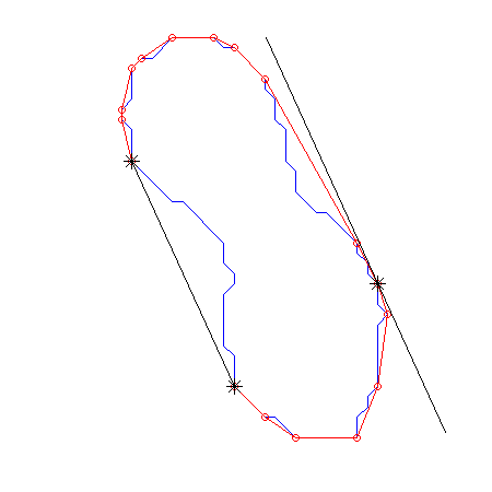
I’ve also added a graphical representation of the calliper:
figure('position',[1000,500,450,450]);
plot([coords(:,1);coords(1,1)],[coords(:,2);coords(1,2)],'b-')
hold on, axis equal, axis off, axis manual
plot([D(:,1);D(1,1)],[D(:,2);D(1,2)],'r-o')
wl = plot([0,0],[0,0],'k-*','markersize',12);
minD = Inf; minV = [];
maxD = 0;   maxV = [];
N = size(D,1);
p0 = N;
p = 1;
q = 2;
while area(D(p,:),D(next(p,N),:),D(next(q,N),:)) > ...
      area(D(p,:),D(next(p,N),:),D(q,:))
   q = next(q,N);
end
q0 = q;
while p~=p0
   p = next(p,N);
   listq = q;                       % p,q is an antipodal pair
   while area(D(p,:),D(next(p,N),:),D(next(q,N),:)) > ...
         area(D(p,:),D(next(p,N),:),D(q,:))
      q = next(q,N);
      listq = [listq,q];            % p,q is an antipodal pair
   end
   if area(D(p,:),D(next(p,N),:),D(next(q,N),:)) == ...
      area(D(p,:),D(next(p,N),:),D(q,:))
      listq = [listq,next(q,N)];    % p,q+1 is an antipodal pair
   end
   for ii=1:length(listq)
      q = mod(listq(ii)-1,N)+1;
      v = D(p,:)-D(q,:);
      d = norm(v);
      if d>maxD
         maxD = d;
         maxV = v;
      end
   end
   pt3 = D(p,:);
   for ii=1:length(listq)-1
      pt1 = D(listq(ii),:);
      pt2 = D(listq(ii+1),:);
      h = height(pt1,pt2,pt3);
      if h<minD
         minD = h;
         minV = pt2-pt1;
         pt4 = pt3 + minV*100;
         pt5 = pt3 - minV*100;
         set(wl,'xdata',...
                [pt1(1),pt2(1),NaN,pt3(1),NaN,pt4(1),pt5(1)],...
                'ydata',...
                [pt1(2),pt2(2),NaN,pt3(2),NaN,pt4(2),pt5(2)]);
         pause(0.5);
      end
   end
end
Now minD and maxD contain the minimum and maximum diameters found, and minV and minV the corresponding vectors.
It is simple to derive the orientation of the two diameters. Computing the diameter perpendicular to the minimum
diameter involves projecting the coordinates of the vertices onto a normalized minV, then looking for the maximum
distance:
maxA = atan2(maxV(2),maxV(1));
minA = atan2(minV(2),minV(1))+pi/2;
minV = minV/norm(minV);
w = D*minV';
minP = max(w)-min(w);
fprintf('Object length: %.2f, at %.2f degreesn',maxD,maxA*180/pi);
fprintf('Minimum bounding box: %.2f by %.2f, at %.2f degreesn',...
        minD,minP,minA*180/pi);
Object length: 37.20, at 53.75 degrees
Minimum bounding box: 21.02 by 36.67, at -26.57 degrees
Note that these distances are between the centres of boundary pixels, and the object itself is typically one pixel wider/longer. The same was true when we computed the Feret diameters from the chain code directly.
The new 'Feret' measurement in DIPimage works essentially this way, as described in
the changelist.