The distance transform, erosion and separability
David Coeurjolly from the Université de Lyon just gave a presentation here at my department. He discussed, among other things, an algorithm that computes the Euclidean distance transform and is separable. The distance transform is an operation that takes a binary image as input, and writes in each object pixel the distance to the nearest background pixel. All sorts of approximations exist, using various distance measures that approximate the Euclidean distance. Using truly Euclidean distances is rather expensive. However, by making an algorithm that is separable, the computational cost is greatly reduced.
David’s algorithm computes the square distance first along each of the rows of the image, then modifies these distances by doing some operations along the columns. In higher-dimensional images you can just repeat this last step along the other dimensions. The operation to modify these distance values sounded very much like parabolic erosions to me, so I just gave this a try.
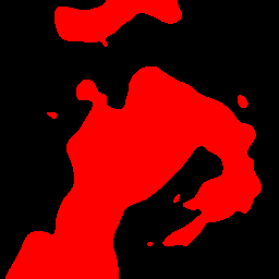
First, we create some test image and compute its distance transform. To execute these commands in MATLAB you need DIPimage.
a = threshold(gaussf(readim,5))
b = dt(a,1,'true')
dipmapping('lin')

By specifying 'true' as an option to the dt function we make sure there’s no errors introduced by speeding up the
computation.
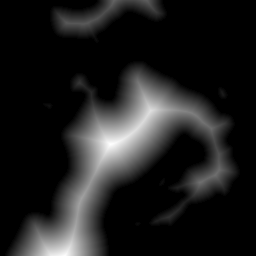
Now, to compute the distance transform using the parabolic erosion, we will generate an image that is Inf everywhere
inside the object. Then we compute the erosion, which will reduce these initial values according to a quadratic distance
to the region with zero values. Note that the erosion with a parabolic structuring element is separable.
c = newim(a);
c(a) = Inf;
c = erosion(c,1,'parabolic');
c = sqrt(c)
dipmapping('lin')
Let’s compare these two results.
any(b~=c)
ans =
     0
So this is an exact result. Is it really faster? To time these operations I use Steve Eddins’ timeit function.
You can get it from MATLAB Central File Exchange.
[Note: this function has since been added to the standard MATLAB toolbox.]
Also, this time I’m using an input image with a really large values instead of Inf. This is just so I can write the
operation as a single MATLAB command: a*1e9 produces a valid input image, but a*Inf produces NaN values where
a is 0. As long as the value used is larger than the square of the maximal distance in the image, this will not
affect the output.
f = @() dt(a,1,'true');
g = @() sqrt(erosion(a*1e9,1,'parabolic'));
timeit(f)
timeit(g)
ans =
    0.0253

ans =
    0.0112
Yes, it is quite a bit faster. But of course, there are approximations that are much faster, and not bad either.
f = @() dt(a,1,'ties');
g = @() dt(a,1,'fast');
timeit(f)
timeit(g)
ans =
    0.0062

ans =
    0.0040
As I wrote this, I decided to check with Rein van den Boomgaard’s PhD thesis (written in 1992). Rein describes parabolic morphology as the morphological equivalent of the Gaussian convolution kernel, because it is the only structuring element that is rotationally invariant and separable. He says that Sternberg (1980) showed that the distance transform can be calculated exactly by erosion with a cone structuring element. He then concludes that you can compute the squared of the distance transform using the parabolic structuring element. This means that this separable algorithm to compute the exact Euclidean distance transform has been around since at least 1992. And I should have known about it!
I think the real advantage of this technique is that a separable algorithm can be split into many threads, and thus obtain a considerable speedup on multi-processor and multi-core computers, as discussed by David today.