Cris’ Image Analysis Blog

A recent question on Stack Overflow really stroke my curiosity. The question was about why MATLAB’s rgb2ind function is so much faster at finding a color table than k-means clustering. It turns out that the algorithm in rgb2ind, which they call ” Minimum Variance Quantization”, is not documented anywhere. A different page in the MATLAB documentation does give away a little bit about this algorithm: it shows a partitioning of the RGB cube with what looks like a k-d tree.

So I ended up thinking quite a bit about how a k-d tree, minimizing variance, and color quantization could intersect. I ended up devising an algorithm that works quite well. It is implemented in DIPlib 3.0 as dip::MinimumVariancePartitioning (source code). I’d like to describe the algorithm here in a bit of detail.

Partitioning a color histogram

The RGB cube is a 3D space where each pixel can be represented as a point. Put all pixels in an image in there, and you get a point cloud. Clustering of these points leads to a partitioning of the RGB cube into cells (or regions, clusters, tiles, whatever you want to call them) that each represent a group of similar colors present in the image. For each cell one can decide on a single color (e.g. the mean) that will represent all colors within that cell. This leads to a short list of colors, a color palette. Next, for each pixel in the image, one finds the cell it falls into, and replaces it with the color chosen for that cell. This transforms the image such that only the colors in the color palette are used. The colors are now quantized, as there are many fewer colors than in the original image. The more cells the RGB cube is partitioned in, the more the transformed image will look like the original image.

This color quantization was a very important technique in the days of 256-color displays, and GIF images, as the quality of the image displayed depended very much on how well the set of 256 colors was chosen.

But note that it is not necessary to go through a clustering process using all pixels in the image. It is much more efficient (typically) to use a color histogram instead. The color histogram is simply a discretization of the RGB cube, where each element is a count of the number of pixels with that color. That is, a color histogram is a 3D array of, say, 32x32x32 or 64x64x64 values, containing pixel counts corresponding to each combination of RGB values. For a normal photograph (today often around 10 or 15 million pixels) this represents a reduction of the number of data points of 40x to 400x.

K-means clustering is the obvious choice for clustering, except that it is quite expensive. Current common methods are the median cut algorithm and a clustering using octrees. The median cut recursively splits the RGB cube along its longest axis, such that each half represents about half the pixels. This leads to a partitioning where each cell represents the same number of pixels. A k-d tree is the data structure used for this algorithm (see below for details). The other popular method builds an octree over the histogram, and merges groups of 8 cells recursively until the right number of cells remain. The least occupied cells are the first to be merged.

K-d trees

K-d trees are a spatial indexing data structure. It is a binary tree (each node has either zero or two children), where the leaf nodes (the ones with zero children) represent the cells of the partition. Each branch node has a threshold value, which operates along one axis. Thus, each node splits the space in two, and all cells are rectangular (or boxes in 3D). Finding the cell that a point in space belongs to is O(log n), for n cells: starting at the root node, follow the left or right child depending on the threshold value stored in the node, until you reach a leaf node.

The k-d tree thus is very flexible in how the space is partitioned, but it cannot generate splits at arbitrary angles, like you can get with k-means clustering. K-means clustering produces a Voronoi tessellation of the space, induced by the k centroids of the cells. Each cell is composed of the points that are closer to the cell’s centroid than to any other of the centroids.

In contrast, in the octree data structure, each node has either zero or eight children, where the children are all the same size and shape. That is, each cell is divided into eighths by splitting it in half along each dimension. This means that the nodes do not need to store a threshold value and direction, but it also means that meaningful clusters will be split, and thus the octree typically requires more cells than an equivalent k-d tree.

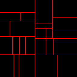
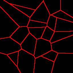
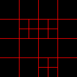
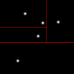
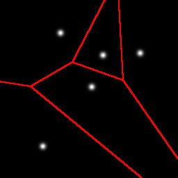
Here are example partitionings of a 2D space into 25 cells using a k-d tree (left), a Voronoi graph (middle), and an octree (actually a quadtree, the 2D equivalent, right):

Minimizing variance

Otsu’s algorithm for finding a global threshold finds a threshold that minimizes the (weighted) sum of the variances of the two classes. This sum is always smaller than the variance of all the data combined. Imagine data with a bimodal distribution, half the data points have a Gaussian distribution with mean and variance , the other half a similar distribution with mean and variance . As long as , then the variance of this data set . Thus, splitting our RGB cube in a meaningful way will reduce the sum of variances along all three axes.

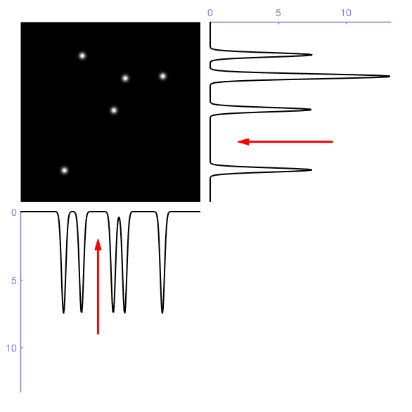
Since the k-d tree always splits along one axis, I figured it makes sense to compute the marginal distributions for a cell (i.e. the projections of the histogram onto each axis), determine the optimal Otsu threshold for each of those projections, and determine which of these three cuts reduces the variance the most. The figure below gives a graphical representation of these marginal distributions and Otsu thresholds in 2D (for the RGB cube you’d add a 3^rd dimension of course). The horizontal cut would reduce the total variance more than the vertical cut, so the horizontal cut is chosen.

This process will allows us to divide the space into two cells. Next, we can repeat this process for each of the resulting two cells, to find the next best cut. But now we also need to choose which of the cells to cut. The more cuts we make, the more cells we will have to choose from. To make this problem tractable, a priority queue is the best approach. Each of the cells is put into the priority queue, with a priority given by how much the sum of variances is reduced by splitting that cell. Now the cell at the top of the queue is always the best one to cut. After cutting it, the two resulting cells are put back into the queue.

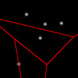
Here is an example partitioning of a 2D space with 5 Gaussian blobs:

As shown earlier, the first cut is a horizontal cut that separates the one blob that is a little bit more isolated than the others. The next cut is a vertical cut of the top cell, again separating one blob from the other three. Next we get another horizontal cut, and finally a vertical cut. Note that these cuts do not need to separate one blob from the group, it is a coincidence that it happened that way in this example.

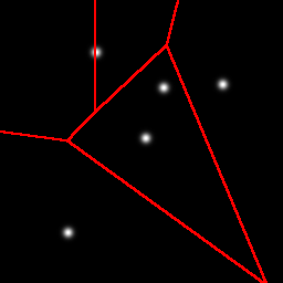
With k-means clustering, using random initialization, you get a different result every time. Sometimes the result is really good, but with data like this you have to get lucky. Many initializations yield poor results, with two or three blobs in one partition, and one blob split into two:

Putting it all together

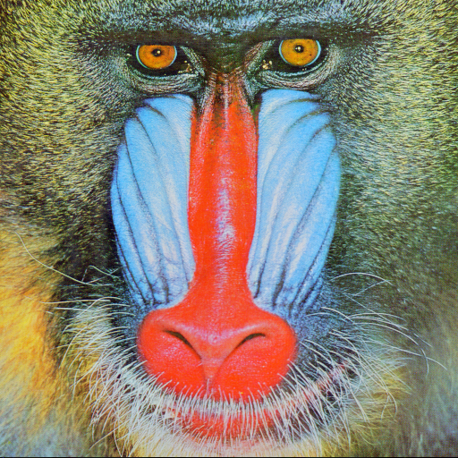
As an example, I’m using the well-known “mandril” image:

Here are the results of using this minimum variance partitioning algorithm on the color histogram with 100³ bins, for 5 colors (left) and 25 colors (right):

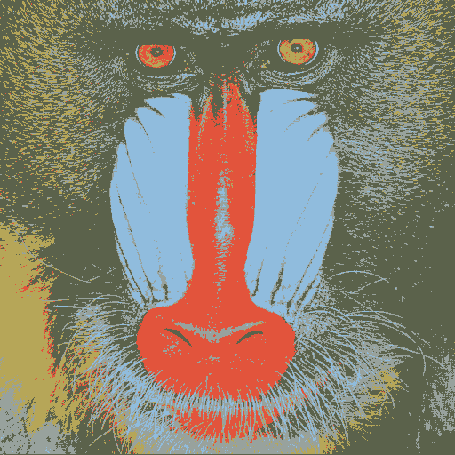
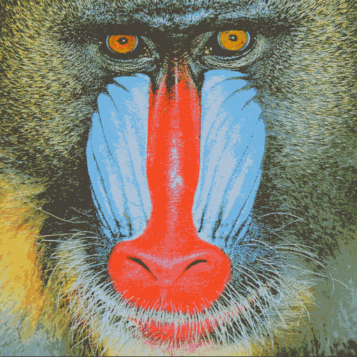
The computation of the 25-color quantized image took 0.05 s on my computer. I find it striking that the image looks so good with only 25 unique colors. For fewer colors, dithering could have improved the results.

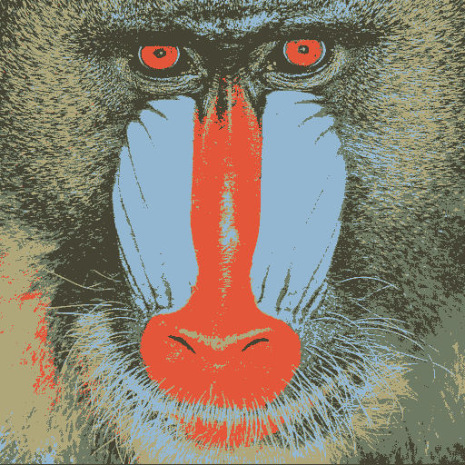
For comparison, this is what the results are with k-means clustering. Running the algorithm multiple times gives slightly different results. The computation of the 25-color quantized image took nearly 5 s, 100 times longer than the minimum variance algorithm.

Which results do you prefer? Do you think that MATLAB’s rgb2ind implements a similar algorithm to this?